Tag Archives: realtime

Measuring the pi3hat r4.2 performance

Last time I covered the new software library that I wrote to help use all the features of the pi3hat, in an efficient manner. This time, I’ll cover how I measured the performance of the result, and talk about how it can be integrated into a robotic control system.

pi3hat r4.2 available at mjbots.com

Test Setup

To check out the timing, I wired up a pi3hat into the quad A1 and used the oscilloscope to probe one of the SPI clocks and CAN bus 1 and 3.

Then, I could use pi3hat_tool incantations to experiment with different bus utilization strategies and get to one with the best performance. The sequence that I settled on was:

  1. Write all outgoing CAN messages, using a round-robin strategy between CAN buses. The SPI bus rate of 10Mhz is faster than the 5Mbps maximum CAN-FD rate, so this gets each bus transmitting its first packet as soon as possible, then queues up the remainder.
  2. Read the IMU. During this phase, any replies over CAN are being enqueued on the individual STM32 processors.
  3. Optionally read CAN replies. If any outgoing packets were marked as expecting a reply, that bus is expected to receive the appropriate number of responses. Additionally, a bus can be requested to “get anything in the queue”.

With this approach, a full command and query of the comprehensive state of 12 qdd100 servos, and reading the IMU takes around 740us. If you perform that on one thread while performing robot control on others, it allows you to achieve a 1kHz update rate.

CAN1 SPI clock on bottom, CAN1 and CAN3 bus on top

These results were with the Raspberry Pi 3b+. On a Raspberry Pi 4, they seem to be about 5% better, mostly because the Pi 4’s faster CPU is able to execute the register twiddling a little faster, which reduces dead time on the SPI bus.

Bringing up the pi3hat r4.2

The pi3hat r4.2, now in the mjbots store, has only minor hardware changes from the r4 and r4.1 versions. What has changed in a bigger way is the firmware, and the software that is available to interface with it. The interface software for the previous versions was tightly coupled to the quad A1s overall codebase, that made it basically impossible to use with without significant rework. So, that rework is what I’ve done with the new libpi3hat library:

It consists of a single C++11 header and source file with no dependencies aside from the standard C++ library and bcm_host.h from the Raspberry Pi firmware. You can build it using the bazel build files, or just copy the source file into your own project and build with whatever system you are using.

Performance

Using all of the pi3hat’s features in a runtime performant way can be challenging, but libpi3hat makes it not so bad by providing an omnibus call which sequences accesses to all the CAN buses and peripherals in a way that maximizes pipelining and overlap between the different operations, while simultaneously maximizing the usage of the SPI bus. The downside is that it does not use the linux kernel drivers for SPI and thus requires root access to run. For most robotic applications, that isn’t a problem, as the controlling computer is doing nothing but control anyways.

This design makes it feasible to operate at least 12 servos and read the IMU at rates over 1kHz on a Raspberry Pi.

pi3hat_tool

There is a command line tool, pi3hat_tool which provides a demonstration of how to use all the features of the library, as well as being a useful diagnostic tool on its own. For instance, it can be used to read the IMU state:

# ./pi3hat_tool --read-att
ATT w=0.999 x=0.013 y=-0.006 z=-0.029  dps=(  0.1, -0.1, -0.1) a=( 0.0, 0.0, 0.0)

And it can be used to write and read from the various CAN buses.

# ./pi3hat_tool --write-can 1,8001,1300,r \
                --write-can 2,8004,1300,r \
                --write-can 3,8007,1300,r
CAN 1,100,2300000400
CAN 2,400,2300000400
CAN 3,700,230000fc00

You can also do those at the same time in a single bus cycle:

# ./pi3hat_tool --read-att --write-can 1,8001,1300,r
CAN 1,100,2300000400
ATT w=0.183 x=0.692 y=0.181 z=-0.674  dps=(  0.1, -0.0,  0.1) a=(-0.0, 0.0,-0.0)

Next steps

Next up I’ll demonstrate my performance testing setup, and what kind of performance you can expect in a typical system.

Log file format (diagnostics part 4)

In parts 1, 2, and 3 I covered some motivation for the updated mjlib diagnostics system and the serialization of individual structures.  In this post, I’ll cover how those structures are written into a file from an embedded system like a robot and how diagnostic tools can access them efficiently.

Goals

The top level goals are:

  • Efficient to write live from an embedded system: The quad A1 generates log data currently at 400Hz, consisting of hundreds to thousands of telemetry data points in every update.  It does this on a relatively low-end raspberry pi 3b+.  The format should be able to support writing data at high rates without a significant CPU burden.
  • Efficient seeking by time and record: Readers of the file should be able to efficiently seek by time in the stream, as well as extract all of a single record without having to process unnecessary data from the log.
  • Self contained: While this property  in the log comes from the underlying mjlib serialization format, it is worth re-iterating here.  All information necessary to return a JSON or CSV like structure for each instance should be present within the log.

Design

The detailed design of the log format is documented at README.md, here I will give a brief summary.

The log consists of a header followed by a series of “Blocks” concatenated together.  The two primary block types are one that contain the schema for an individual record and one for the data.  For a given record the schema will only be present once in the log, typically near the beginning.  The data block, contains a single serialized instance of the record, along with some optional flags and data.  The optional flags include a timestamp, a checksum, whether the data is compressed, and a pointer to the most recent data block for this record.

Another block is the SeekMarker block, which contains a timestamp and a 64 bit long unique-ish byte code and a checksum.  When readers need to perform random seeks in the log, they can binary search to an arbitrary byte offset, then search to find an instance of this unique code.  If it is present in conjunction with the necessary header and a validated checksum, it can be assumed that the framing has been recovered and the time for that point in the log.

Finally, there is an Index block, written at the very end of the log.  This includes pointers to the schema entries for all records in the file, as well as the most recent data block for that record.  That allows readers to find the set of records in a log, and extract a single record (albeit backwards) from the log while reading no extra data.

Future extensions

Most of the entities in the log have flag bitmasks to control additional future features or extensions.  Current readers throw errors when unknown bits are discovered, which makes it safe to almost arbitrarily modify the log structure at the expense of forward compatibility.

The mostly likely extensions are related to compression.  The current per-data compression format is snappy, from google.  It is fast, but has relatively poor compresson performance.  At some point, I’d like to switch to Zstandard, which has even better runtime performance, much better compression performance, and supports incremental dictionary manipulation.  I have actually integrated into in a test manner into the C++ writer and reader and the effort was trivial, however the other languages that I support, python and TypeScript are more challenging.  With snappy, there are operating system provided packages that work just fine in Debian and Ubuntu, but not so for Zstandard.  Bazel has rules that support pulling in pip packages for python and npm for TypeScript, but both of those mechanisms don’t have very straightforward support for the recursive WORKSPACE workarounds I am using now.  For now, it is easiest just to stick to snappy.

Next

Now that we have the data structures out of the way, I’ll move on to the tools that use them!

Failing more gracefully

My outdoor filming for the project update video was cut short when the machine cut power to the motors, fell down, and one of the legs snapped off.  Fortunately, I already had plenty of footage when that happened, so it didn’t really impact the video.

dsc_1541
Robot down

dsc_1540-1
Nice infill shot

First, this demonstrates the not too surprising fact that this particular part of the leg design could use to be improved.  Second, and the topic of this post, is improving what the machine does when the inevitable failure does occur.

What happened — just the facts ma’am

In this particular instance, I had been running the machine outside continuously outside for an hour or so on a relatively warm day.  This iteration of the servos has basically no heatsinking whatsoever on the servo control board.  With the gearboxes, it isn’t necessary for short duration or low power testing.  However in this case, one of the servos eventually reached its temperature limit and entered a fault state.

As implemented now, any individual servo that hits a hard fault immediately cuts all power.  Also, at that time, the overall gait control, upon sensing any servo failure, immediately cuts power to all the other servos too.  As you can imagine, when a machine that weights 10kg loses all power to all joints with a few milliseconds, it falls down pretty hard.

Areas to improve

There are of course many areas of improvement which this event demonstrates.  One, the servos need better thermal properties.  This was known, and I hope to address in the second revision where I can heatsink the controller properly.  Second, the leg should be strong enough to handle falling down.  And third, it would be nice, if it could, if the machine would do something more graceful when continuing on in a controlled manner isn’t possible.

I tackled that third step right now in two phases.  First, I set up an optional communications watchdog in the servo.  If control commands aren’t received in a timely manner, the servo enters a new mode where it merely commands a zero velocity with no position control at all.  This means that if the control software segfaults, or the primary computer goes out to lunch, the machine will gently lower to the ground rather than dropping like a rock.

Second, I modified the control software’s reaction to an individual servo fault.  Now, it commands this new zero-velocity state of all unfaulted servos so as to minimize the amount of damage done to the overall machine.  If only one or two servos have faulted, this will still result in a relatively gradual let down.

Here’s a quick video demonstrating the two failure types:


Improving the moteus update rate, part 4

In part 1, part 2, and part 3, I looked at what was limiting the update rate of the moteus controller when built into a quadruped configuration and how to improve that.  Now, it is time for the final demonstration!

That video was shot with a 150Hz overall update rate.  The plot shows the commanded and actual position of the three joints in the front right leg, although not all to the same vertical scale.  Updating the servos themselves only used about 3.5ms per cycle, but the gait logic used another 1-1.5ms, which made hitting 200Hz not super reliable, thus running at 150Hz.

Future work

I would still like to be able to perform 1kHz full system updates.  These experiments have let me come up with a plan that I think will achieve that with plenty of margin from the servo side in the next revision.

  • Switch the controllers to use FD-CAN:  I had initially not used CAN as the communication mechanism because I didn’t want to be limited to 1Mbps and 8 byte frames.  However, recent STM32 controllers come with FD-CAN support, which allows up to 64 byte frames and 8Mbps.  The hardware FD-CAN receiver implements CRCs for free, should be more reliable, and manages some amount of pre-filtering and processing, which should further reduce the turnaround time of querying a device.
  • Integrate with the host computer over SPI: While I was able to make serial work by busy loop polling on a dedicated CPU, the SPI bus has an even higher possible bitrate and even if its kernel driver is just as problematic, it can still be polled in the same way.
  • Operate 4 separate busses:  This will be done by having probably 2 STM32’s on the host computer daughterboard, each managing two busses.  This way each leg will have its own CAN bus.


Improving the moteus update rate, part 3

Back in part 1 and part 2, I looked at problems that limited the rate at which the host computer could command the full quadruped and some of the solutions.  Now, in part 3, I’ll cover more of the solution.

More solution steps

Previously, I switched to using PREEMPT_RT, switched bridging strategies, and optimized the turnaround of the individual servo.  Now, I’ll move on to optimizing the host software.

4. Host C++ software micro-optimizations

The primary contributor in the host software to the overall update rate is the time it takes to turn around from receiving a reply from one servo, to sending the next command.  I first did some easy micro-optimizations which came up in profiling.

  • error_code: My implementation of error_code with strings attached was doing lots of string manipulation even when no one asked for it.  Fixing that saved a fair amount of time throughout.
  • Memory allocation: There were a few sites in the code that generated packets where a persistent buffer could be used each time, instead of having to allocate a fresh one.

5. boost::asio

The host software was using boost::asio to interact with the serial port.  It is high performance for what it does, allowing multiple external operations to happen in the same thread, but necessarily relies on an epoll loop and non-blocking write operations.  These aren’t particularly fast in the linux kernel, and the best turnaround time on the rpi I could achieve with asio was around 80us.

I implemented a standalone proof of concept which just uses a single thread to read and write to the serial port in a blocking manner.  Doing that allowed me to get the turnaround down to around 30us.

6. Protocol design

The register protocol that is used for high rate control had one opcode for setting a single register, and another for setting multiple consecutive ones.  The multiple consecutive one requires an additional byte to identify how many registers are set.  The same thing is true for queries.

I shaved a byte off of the common case of both by allowing writes and reads of up to 3 registers to encode their length in the primary opcode.

With that change, the full query packet to each servo was 23 bytes, and the full reply packet was 28 bytes.

7. Linux serial driver latencies

With the blocking thread approach from step #5 and that thread set to real-time priority, the average turnaround was indeed 30us.  However, when run in the full control software (which does other processing as well), occasionally latencies would be in the several millisecond range.  Also, since the PL011 on the raspberry pi only has a 16 byte FIFO, reading any frames larger than that was unreliable, as the kernel didn’t always get around to servicing things fast enough.  Even with sub-16 byte frames, and a blocking reader, the kernel would still delay reads by a millisecond or so sometimes.  I believe this is because the PL011 only provides interrupt notification on even 4 byte boundaries of its FIFO, and otherwise relies on the kernel to poll it.

Well, I can poll too, so I fixed this by just disabling the kernel’s serial driver, opening up “/dev/mem” and polling the IO memory of the controller manually in a busy loop from a RT thread.  This let me get turnarounds down to 4us, and also let me receive packets of arbitrary length without loss.  See https://github.com/mjbots/mjmech/blob/master/mech/rpi3_raw_uart.h and https://github.com/mjbots/mjmech/blob/master/mech/rpi3_raw_uart.cc

8. Linux scheduling latencies

With the above changes, the serial port was doing fine, but linux still had problems scheduling the primary process to run with less than 1ms precision, even when it was RT priority.  To solve that, and make the serial thread a bit better performing too, I used the “isolcpus” feature of linux to exclude 2 of the 4 raspberry pi processors from normal scheduling.  Then the main thread of the application got processor 3, and the serial thread got processor 4.  With those changes, the time required to poll the full set of 12 servos is rock solid.  Here’s a plot showing the cycle time required to poll a full set of telemetry data  (but not command them, which adds a bit more time per query but doesn’t affect the variability).

20190919-improved-latency-jitter.png

Next steps

And in the next and final post of this series, I’ll demonstrate the final result, showing all of these changes are integrated into the primary control software.


Improving the moteus update rate, part 2

Back in part 1, I looked at the driving factors that limited the update rate of the full quadruped.  Now in part 2, I’ll cover the first half of the solution.

Background

To begin with, there were two major paths that I could take based around the network topology.  In one path, I would remove the active bridging capability from the junction board, and rely on the Raspberry Pi to drive all the servos directly, and in the other the active bridge would stick around.  There were a number of key disadvantages to both approaches:

Passive bridge: In this model, the raspberry pi has no choice but to rapidly turn around 12 separate queries and responses.  There is no hope for parallelization.

Active bridge: Here, the junction board’s STM32 can offload the multiple queries.  However, there are two big downsides.  The first are that the data must flow across 2 separate 485 busses.  The second, and possibly more problematic, is that it only works out better if the junction board can stream a large amount of data consecutively to the raspberry pi.  In my previous experiments, I had run into what I believe was a kernel bug that killed the serial port until a power cycle upon receive overruns.  Debugging that could easily be a large project.  Implementing the active bridge would also be a lot of work, as I don’t currently have a protocol client that runs on the STM32.

My initial back of the envelope calculations, surprisingly, indicated that both approaches could potentially get up to 250 or 300Hz with sufficient margin to still do other things.  I had expected that parallelization would win the day, but it turned out that duplicating the data across both busses had the potential to completely negate that advantage.

Solution steps (first half)

1. RT_PREEMPT

The first thing I did was to switch to using a RT_PREEMPT enabled kernel with the governors set to performance.  This by itself reduced the Raspberry Pi’s reply to query turnaround from 200us to 100us.  I wanted to at this time also upgrade to the 4.19 kernel, as I hoped that it would have some fixes for high serial rates.  However, it doesn’t look like anyone has a RT enabled 4.19 kernel that supports USB and ethernet, both of which are moderately useful on a board with not many other interfaces.

2. “Passive” bridging

In lieu of spinning a new board right away, I instead modified the firmware of the junction board to remove almost all functionality and instead just busy loop shoving individual bytes around between the interfaces.  It is fast enough to just barely be able to achieve this at 3Mbit if interrupts are off.  The downside is that the IMU won’t be usable.  To fix that, I’ll have to spin a new board that just passively wires all the busses together and dangles the STM32 off the bus like any other node and hope that the star topology won’t matter over such short distances.

Doing this removed the double transmission penalty, as well as the additional 90us latency in the junction board on all transfers.  This, combined with RT_PREEMPT, got the overall cycle time down to about 6727us, or ~150Hz.

3. Controller turnaround time

Next, I started in on the moteus firmware, in order to improve the turnaround time between when a query is sent, and when the corresponding reply is generated.  This resulted in many optimizations throughout the code.  The first set were made to the primary control ISR, which runs at 30kHz currently.  Tiny improvements here make everything else run much faster.

  • Constructors: The ARM gcc toolsuite, regardless of the optimization level, seems to implement a constructor of an all zero structure as a call to memset.  This is true even if the structure is a small number of bytes.  There were several places in the firmware where a structure was zeroed out by calling its default constructor.  Switching that to a “clear” method which manually assigned all the fields drastically reduced the time spent there.
  • Appropriate types: When calculating a smoothed velocity, the filter was using an int64_t as an intermediate variable, which is not very efficient on an ARM.  Nothing more than an int32_t was actually needed.
  • fmod: I was wrapping between zero and two pi by using fmod.  The cases where wrapping occurs were never more than one or two phases off, so just dividing and truncating was much faster with no appreciable loss of precision.
  • Pre-computing some variables: Some of the calculations done in the ISR were repeated unnecessarily, so now they are on re-computed upon a configuration change.
  • Make debug output optional: The moteus board has a high rate RS422 debug output, which is only rarely used.  I added a configuration knob to turn it off when not in use.
  • SPI overhead: I was using the ST HAL API to access the position sensor over SPI.  I still do that for setup, but now just twiddle the raw registers to do the actual transfer, which saves a little bit of overhead in the HAL.
  • SPI frequency: The AS5047P has a nominal SPI frequency limit of 10MHz.  I asked the HAL for 10MHz, but the closest it could actually do was 6MHz.  I decided to brave some flakiness and upped it to 12MHz to shave another microsecond off.

After these changes, the ISR uses around 7-8us when stopped, and around 13us per iteration when in position control mode, or around 40% of the CPU budget.

Next I made more optimizations to the software which runs in the main loop:

  • StaticFunction: I was using a home-grown solution to a bounded size type-erased function callback that wasn’t particularly fast.  I switched it out for the SG14 inplace_function from github, modified to allow shrinking to a smaller type.  That sped up everything in the main loop by a fair amount.
  • Protocol parsing: A number of steps in the protocol parsing and emitting eventually delegated to a call to “memcpy” into a particular type.  I broke some abstractions so that all that parsing and emitting eventually compiles down to just loads and stores.
  • Reply encoding: The RS485 register protocol allows clients to query multiple consecutive registers.  As a shortcut, the server was responding to those with a series of single register replies.  I fixed that by implementing sending multiple replies at once to shave off a few bytes and some processing.

I experimented with using the STM32F446’s built in CRC unit, however it only implements a fixed CRC-32 variant.  So updating that would have required reflashing all my bootloaders.  Using that is probably best taken by updating to an STM32F7 or STM32G4 which have more configurable CRC units.  I also tried hand assembling an optimized version of the CCITT16 checksum I was using, but was only able to achieve the same 8 cycles per byte that boost already had.

With all of these changes, the average turnaround time for a single servo was down from 140us to in the 70-80us range for a full control update.

Next steps

Coming up, in part 3, I’ll cover the remainder of the steps I took to improve the overall update rate.


Improving the moteus update rate, part 1

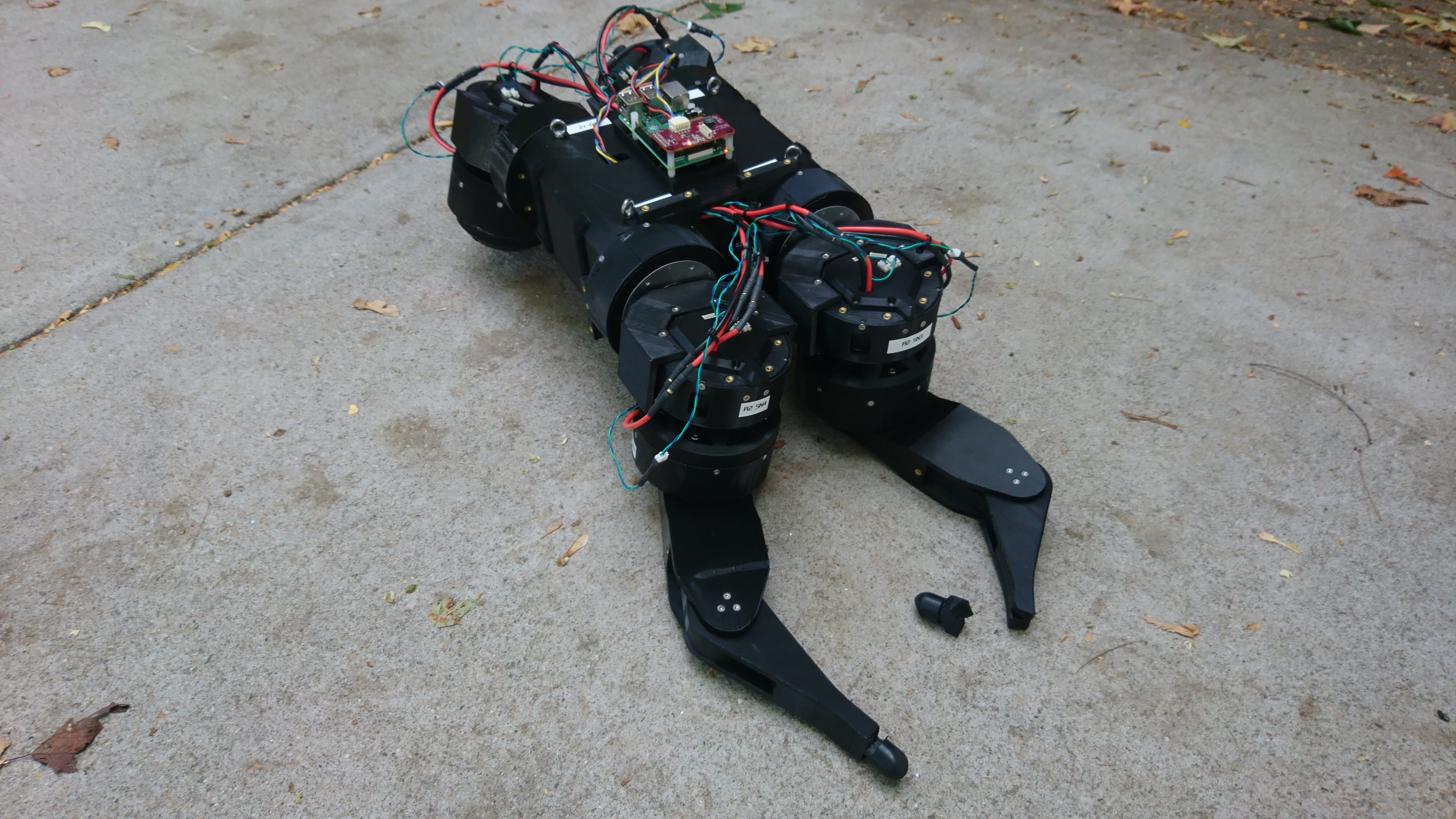
The moteus brushless controller I’ve developed for the force controlled quadruped uses an RS485 based command-response communication protocol.  To complete a full control cycle, the controlling computer needs to send new commands to each servo and read the current state back from each of them.  While I designed the system to be capable of high rate all-system updates, my initial implementation took a lot of shortcuts.  The result being that for all my testing so far, the outgoing update rate has been 100Hz, but state read back from the servos has been more at like 10Hz.  Here I’ll cover my work to get that rate both symmetric, and higher.

In this first post, I’ll cover the existing design and how that drives the update rate limitations.

Individual contributors

There are many pieces that chain together to determine the overall cycle time.  Here is my best estimate of each.

RS485 bitrate

The RS485 protocol that I’m using right now runs at 3,000,000 baud half duplex.  That means it can push about 300k bytes per second in one direction or the other.  While the STM32 in the moteus has UARTs capable of going faster than that, control computers that can manage much faster than 3Mbit are rare, so without switching to another transport like ethernet, this is about as good as it will get.

This means that at a minimum, there is a latency associated with all transmissions associated with the amount of data, which is roughly bytes * 10 / 3000000.

Servo turnaround

The RS485 protocol moteus uses allows for unidirectional or bidirectional commands.  In past experiments, all the control commands were sent in a group as unidirectional commands, then the state was queried in a series of separate command-reply sequences.  The firmware of the moteus servo currently takes around 140us from when a command finishes transmission and the corresponding reply is started.  The ideal turnaround for a bare servo is then (txbytes * 10 / 3000000) + 140us + (rxbytes * 10 / 3000000).

IMU junction board

The current quadruped has a network topology that looks like:

imu-junction-block-diagram

The junction board is an STM32F4 processor that performs active bridging across the RS485 networks and also contains an IMU.  This topology was chosen so that the junction board could query both halves of the quadruped simultaneously, then send a single result back to the host computer.  However, that has not been implemented yet, thus all the junction board does is further increase the latency of a single command.  As implemented now, it adds about 90us of latency, plus the time required to transmit the command and reply packets a second time.  That makes the latency for a single command and reply now: 2 * (txbytes * 10 / 3000000) + 110us + 90us + 2 * (rxbytes * 10 / 3000000)

Raspberry pi command transmission

As mentioned, the current system first sends new commands to the servos, then updates their state.  When sending the new commands, the existing implementation makes a separate system call to initiate each servos output packet.  Sometimes the linux kernel groups those together into a single outgoing frame on the wire, but more often than not those commands ended up being separated by 120us of white space.  That adds 12 * 120us of additional latency to an overall update frame.  So, 12 * 120us = 1440us

Raspberry pi reply to query turnaround

During the phase when all 12 of the servos are being queried, after each query, the raspberry pi needs to receive the response then formulate and send another query.  This currently takes around 200us from when the reply finishes transmission until when the next query hits the wire.  This is some combination of hardware latency, kernel driver latency, and application latency.  It sums up to 200us * 12 = 2400us

Packet framing

The RS485 protocol used for moteus has some header and framing bytes, that are an overhead on every single command or response.  This is currently:

  • Leadin Framing: 2 bytes
  • Source ID: 1 byte
  • Destination ID: 1 byte
  • Payload Size: 1 byte for small things
  • Checksum: 2 bytes

That works out to a 7 byte overhead, which in the current formulation applies 12x for the command phase, and 48 times for the query phase.  12x for the raspberry pi sending, 12x for the junction board sending, and 24x for the combined receive side.  That makes a total of (12 + 48) * 7 = 420 bytes * 10 / 3000000 = 1400us

Data encoding

In the current control mode of the servo, a number of different parameters are typically updated every control cycle:

  • Target angle
  • Target velocity
  • Maximum torque
  • Feedforward torque
  • Proportional control constant
  • Not to exceed angle (only used during open loop startup)

The servo protocol allows each of these values to be encoded on the wire as either a 4 byte floating point value, or as a fixed point signed integer of either 4, 2, or 1 bytes.  The current implementation sends all 6 of these values every time as 4 byte floats.  Additionally two bytes are required to denote which parameters are being sent.  That works out to: ((6 parameters * 4 byte float + 2) * 12 servos * 2 for junction board * 10) / 3000000 = 2080us

The receive side returns the following:

  • Current angle
  • Current velocity
  • Current torque
  • Voltage
  • Temperature
  • Fault code

And in the current implementation all of those are either sent as a 4 byte float, or a 4 byte integer.  That makes ((6 parameters * 4 bytes + 2) * 12 servos * 2 for junction board * 10) / 3000000 = 2080us

Overall result

I put together a spreadsheet that let me tweak each of the individual parameters and see how that affected the overall update rate of the system.

I made a dedicated test program and used the oscilloscope to monitor a cycle and roughly verified these results:

overall-latency

Thus, with a full command and query cycle, an update rate of about 80Hz can be achieved with the current system.

Next up, working to make this much better.