Tag Archives: tplot

Balancing gait in 2D

After getting a gait which looked like it could balance across the leg support line in 1D, I needed to extend that to 2D and try it out on the robot.

Extension to 2D

Extending this to two dimensions wasn’t too bad. I just did a bunch of geometry to follow the path traced out by a given 2 dimensional velocity and rotation rate, intersected with a line segment:

Given this function, the logic to select a swing target is basically the same as in the 1 dimensional case. We now create two “virtual legs”, which consist of two feet ganged together and produce a single support line. At each time instant when all legs are in stance, we look at the time remaining until each of the virtual legs would cross the center of mass at the current velocity. As soon as one hits the half-swing point, we start a swing.

As part of this, I extended tplot2 to be able to render the target location of each swing.

Remaining niggles

Once I had an actual robot to test it out on, I found a few other minor problems. When selecting the target for a foot swing, the 1 dimensional case just used the current velocity to move the leg far enough past the pickup point. That doesn’t work out all that well in heavy acceleration though, resulting in very short stance times. What worked much better was to use the expected velocity at the end of the next stance window. That provided much more consistent stance spacings even when accelerating or decelerating.

I still haven’t come up with a great solution for turning in place, for which the entire concept of estimating distance to the balance point doesn’t make sense. Right now, I just rely on the maximum stance time to ensure the legs eventually step in that scenario and don’t extend beyond their physical limits. I’ll probably eventually add a “time to infeasible geometry” criteria to handle that.

Testing it out

While there is still a lot of remaining work, this increased the maximum possible speed of the machine by at least a factor of 2, and the feasible acceleration by a factor of 10 or so. In the video below, I’ve got some clips of the robot walking around at 0.5m/s. That’s not too fast, but is more than a body length per second which counts for something.

First steps towards more dynamic gaits

Now I’ve got a machine, the mjbots quad A1, which is capable of dynamic motions, but the only gait which takes advantage of these capabilities is the pronking one. That gait has the benefit that the dynamics are very simple. The entire time that that robot is in contact with the ground, it is in contact with all 4 legs, so in that regime it is fully controllable. Since it is fully controllable up to the point of lift-off, we can ensure that there is basically zero rotational rate while the machine is mid-flight, which means that it lands with all four legs largely at the same time. Of course, pronking isn’t a very fast or efficient way of getting anywhere, so I wanted to make the first steps… I guess pun intended, towards improving the more general walking algorithm to make the machine move faster in a more robust manner.

My previous solution

As described here, the gait I was using previously is conceptually very similar to a static IK based gait. The sequencing works by picking up and moving opposing pairs of legs in an alternating fashion. As opposed to a purely IK based solution, the inverse dynamics are accounted for. During the motion, each servo is commanded with appropriate velocities to achieve the end foot velocity profile and appropriate forces are commanded to result in a ground reaction force that matches the mass of the robot.

However, there are many things this doesn’t take into account. Among them are the linear and rotational inertia of the overall machine, the torque that the gravity vector exerts on the center of mass, and the dynamics of the legs themselves, which are assumed massless. It also only uses the high rate feedback from the servos in a very limited way, only to apply a 3D force and velocity command. Thus it completely ignores if a leg strikes the ground early either because of an obstacle or because the machine tipped, or if it strikes the ground late/never because of a depression or hole. Because of all this, it also requires periods where all four legs are on the ground simultaneously in order to maintain stability.

In this simple gait on flat ground, most problems manifest as the robot tipping during the flight phase, resulting in one flight leg striking early, which then results in a high angular rate correction as the controller tries to jam it back to the desired position. This can end up with uncontrolled oscillation of the robot in a wide range of hard to define operating conditions. Note, this is roughly the same problems that most IK based gait engines have, such as on the original Super Mega Microbot.

You can make this gait work passably if you carefully tune things and stick within a limited acceleration and terrain operational envelope, but overall it is rather fragile.

Plan

I’m not planning on tackling all of these problems in one go, or just out and out copying another solution, but intend to take small documentable steps towards a more capable machine. Up next I’ll describe my first baby steps towards this, where I look to manage the gravity torque during the flight phase to keep the machine stable even under acceleration.

Improved swing trajectory

Now that I finally have tplot2 working sufficiently to diagnose problems in 3D, it is time to start actually fixing those problems. The first obvious thing I noticed when watching data replay was that the legs scooted around a lot after making contact with the ground. Absent 3D visualization, I knew something was wrong, but couldn’t easily tell what.

Diagnosing the first problem

Once I was able to plot the commanded position and velocity trajectory, I could clearly see a number of problems. For one, the trajectory was not terribly achievable. The velocity jumped in a discontinuous manner between different phases of the swing cycle, which resulted in large tracking errors when moving the physical legs:

Also, there are those odd periods near the downturn where the commanded Z velocity goes to exactly zero for a while, then resumes its downward trend in a non-physical manner.

When I first wrote the simple walk cycle, I didn’t spend a whole lot (well almost zero) time debugging it, as I didn’t have appropriate debugging tools. Clearly it wasn’t working and something better needed to be done.

Updated swing trajectory

While not the entirety of the problem by any stretch, I figured fixing the swing trajectory was a fine first step that would be mostly independent of any other resolutions. I wanted the swing phase of the leg movement to have a few properties:

  • Continuous velocity profile (I don’t care about jerk)
  • When lifting off and touching down, maintain the ground velocity for a brief period of time
  • For now, I’m not doing whole body control, so the trajectory can be scripted, and it is acceptable to lock in the target position at foot liftoff time

I decided to tackle the problem independently in the Z axis and in the XY plane. In both cases, the approach is based on piecewise cubic bezier curves. In one dimension, these curves have a continuous first and second derivative, but only the position and first derivative are controllable.

For the equation:

x=t^3 + 3 * (t^2 * (1 - t))

The position, velocity, and acceleration are as follows:

Z axis

To generate the Z trajectory, we’ll just stick two of these back to back in a mirrored fashion, so the Z height raises to a peak at the halfway point, then lowers back to the original value with a continuous velocity reaching exactly 0 velocity at the touch down point. That makes the overall Z trajectory look like:

X-Y Plane

In the X-Y plane, I broke up the swing into 3 piecewise sections. The first is a constant deceleration profile from the initial velocity to 0, and the last section is a constant acceleration profile from 0 to the target velocity. The middle section is just a single cubic bezier curve independently applied in the X and Y axes. A sample trajectory (with velocities shown as vectors), might look like:

Then to put the Z and X/Y pieces together, here’s a plot in the XZ plane of a similar system:

So yes, it seems to be doing what we want in that the velocity is continuous in all 3 axes — we lift off gradually, perform our swing, then set back down gradually.

Testing on the robot

Well, I actually tested it first in simulation, but where’s the excitement in that! Here’s what the tplot2 video looks like with the new leg trajectory in a slightly stuttery GIF:

The green and blue feet in the 3D view show that the legs track the control points well, and that 2D plots shows that yes, the Z position and velocity are smooth and continuous as we desired.

Primitive derived fields in tplot2

One of the features that I wanted to get working in the newer tplot2 is some facility for rendering values which are calculated from the things in the log, even if not directly logged there. Straightforward simple cases would be things like the lengths of vectors, unit conversions, or quaternion to euler angles. You could imagine needing arbitrarily complex values plotted after the fact.

In past systems I’ve designed, I built in a generic scripting interface to allow arbitrary things to be plotted. I’d like to do that here as well eventually, but in the short term I had a need to plot the total normal force exerted on the ground by all stance legs. And I didn’t want to spend a lot of time designing a generic mechanism. Thus, I rigged up a very primitive C++ only mechanism, where a function can be registered which returns an arbitrary serializable structure. That is then rendered in the tplot2 tree view in a dedicated area, and has a pretty “hacky” way of getting its values on the plot if necessary.

With some luck, I’ll get a more robust mechanism in the future, but this works for now.

Video and telemetry synchronization (diagnostics part 8)

This is part of a continuing series on updated diagnostic tools for the mjbots quad A1 robot.  Previous editions are in 1, 2, 3, 4, 5, 6, and 7.  Here I’ll be looking at one of the last pieces of the puzzle, synchronizing the video with the rest of the telemetry.

As mentioned previously, recording video of a robot running is an easy, cheap, and fast way to provide ground truth information on all of the sensors and actuators.  However, it is only truly useful if it can be accurately synchronized in time to the other telemetry streams for the robot.

Options

This was part of the puzzle that I spent a long time thinking about before I got started, as there are several possible options that seemed like they could maybe work:

Visual

The concept here would be to put an LED beacon on the robot that is visible from all angles.  It could strobe a synchronizing pattern, like the output from an LFSR which could be identified in the subsequent video frames.

Pros: This should be able to give frame accurate synchronization, and works even for my 1000 fps camera which can’t record audio.

Cons: It is hard to find a good place to mount a light which could be observed from all angles.  The top is the best bet, but I have plans to attach further things there, which would then render synchronization infeasible.

Audio

In this concept, I put a microphone on the robot and have it record audio of the environment during its run.  Then standard audio synchronization algorithms can be used to align the two streams.  I actually included a microphone on the most recent version of the pi3 hat to potentially use this approach.

Pros: This has no visibility requirements, and should be able to give synchronization accuracy well under a single frame of video.

Cons: Getting the microphone data off the pi3 hat was looking to be moderately annoying, as the STM32 which it is connected to is already streaming IMU and RF data back to the robot over its single SPI bus.  When I brought up the board, I verified I could get 1kHz audio off, but that isn’t enough to be useful.

IMU

This was the idea I had last, and what I am using now.  Here, I slap the side of the robot in a semi-random pattern during the video.  That results in an audio signature in the video, as well as lateral accelerometer readings.

Pros: No additional hardware or software is required anywhere on the robot.

Cons: This has worse accuracy than pure audio, as the IMU is only sampled at 400Hz and doesn’t perfectly correspond to the audio found in the video.

Implementation

I took a stab at the IMU version, since it looked to be the easiest and still gave decent performance.  I made up a simple python tool which reads in the robot telemetry data, the audio stream of a video file, and lets the user select rough ranges for the audio and video streams to work from.

It then uses scipy.signal.correlate to do its best job of finding an alignment that best matches both data streams, producing a plot of the alignment.

20200515-video_aligner

As you can see, the audio rings out for some time after the IMU stops its high frequency response, largely due to the mechanical damping of the robot.  However, it is enough for the correlation to work with and give frame accurate results.

3D rendering in tplot (diagnostics part 7)

In previous posts of this series, I covered some diagnostics improvements I’ve made to help work on more advanced gaits for the mjbots quad A1 (1, 2, 3, 4, 5, 6).  This post will cover the last major new piece of diagnostics I added to tplot2, 3d rendering of telemetry data.

3D rendering

While it should be obvious, I’ll give a little exposition.  tplot2 in its state prior to this could show a “tree view” of all data logged in numeric form.  It had a “plot view” which let you plot any single floating point scalar vs time.  As of recently, it could also render video associated with a given point in time in the log.  However, as anyone who has ever tried to debug a 3d dimensional software application, much less a 3d dimensional robot, can attest, debugging with scalar numbers and time plots is only productive for a very limited range of problems.

I’ve been wanting to extend my plotting tools with 3d rendering for some time, and now have gotten around to a minimal first pass.  The logic itself isn’t terribly complicated.  A separate GL Framebuffer object is created in order to render into a texture, then pretty standard GL vertex and fragment shaders are used to render some triangles and lines.  Initially, I’m just doing the robot body, the commanded and actual feet positions, speeds, and forces, and an estimate of the ground underneath them.

20200515-tplot2-3drender

20200515-tplot2-3drender-video

While there is a lot of room for improvement here, both in terms of the visual quality of the existing renderings, and new features that could be rendered, this is already proving itself to be invaluable in diagnosing longstanding problems with the gait motion.

Video in tplot2 (diagnostics part 6)

This is part of a continuing series on diagnostics tooling for the mjbots quad series of robots.  The previous editions can be found at 1, 2, 3, 4, and 5.  Here, I’ll cover the first extension I developed for tplot2 to make it more useful to diagnose dynamic locomotion issues.

Background

Diagnosing problems on robots is hard.  The data rates are high, sensing is imperfect, and there are many state variables to keep track of.  Keeping track of problems that are related to erroneous perception are doubly challenging.  Without a recording of the ground truth of an event, it can be hard to even know if the sensing was off, or if some other aspect was broken.  Fortunately, for things the size and scope of small dynamic quadrupeds, video recording provides a great way to keep a record of the ground truth state of the machine.  Relatively inexpensive equipment can record high resolution images at hundreds of frames a second documenting exactly where all the extremities of the robot were and what it was doing in time.

To take advantage of that, my task here is to get video playback integrated into tplot2, so that the current image from some video can be shown on the screen synchronized with the timeline scrubber.

Making it happen

Here I was able to use large amounts of the code that I developed for the Mech Warfare control application.  I already had the ability to render ffmpeg data to an OpenGL texture.  The missing pieces I needed were getting that texture into an imgui window and adding seek support.

The former was straightforward.  imgui has a Image and ImageButton widgets which allow you to draw an arbitrary OpenGL texture into an imgui widget.

The latter was a little more annoying, only because the ffmpeg API had a slightly unusual behavior.  Even after av_seek_frame was called, one frame from the old point would still be emitted.  This confused my seeking logic, possibly causing it to ignore frames.  However, after discarding that one stale frame, it worked seemingly just fine.

20200515-tplot2-video

Next I’ll cover the last major piece I added to tplot2 to help with issue diagnosis.

tplot2 (diagnostics part 5)

In previous posts, (1, 2, 3, 4), I covered the updates I made to the underlying serialization and log file format used in mjlib and the quad A1.  This time I’ll talk about the graphical application that uses that data to investigate live operation.

History

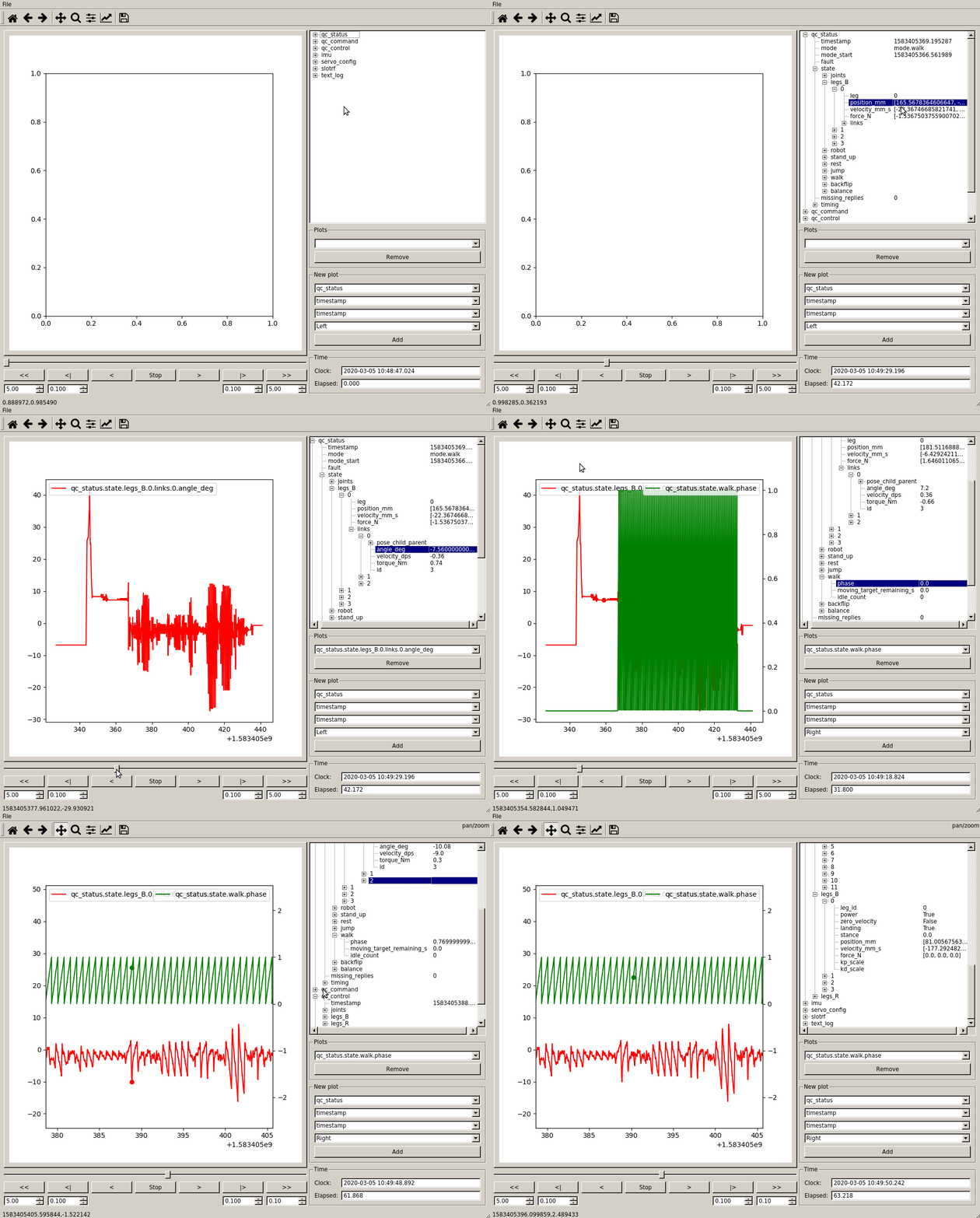
You might note the “2” in the name and realize that yes, this is the second incarnation in the mjmech repository, tplot being the initial.  The original tplot.py was a largely a one-day hack job that glued together the python log bindings I had with matplotlib.  It provided a time scrubber, a tree view, and a plot window where any number of things could be plotted against one another.

20200514-tplot

It did have a number of problems:

  • Speed: The original tplot read the entirety of the log into memory before letting you view any of it.  Further, while reading it into memory, it converted everything into python structures.  This took some time for even relatively short logs.
  • Coding efficiency: This might seem paradoxical, but developing GUIs in PySide still takes a decent amount of time, even if you don’t care what they look like at all.  Either you have all the overhead of using Qt Designer and thus have to manage either UI file loading or compiling, or you design the layouts in code and have mysterious layout issues because the exact construction requirements to get valid layouts are very hard to determine without looking at the QT source.  There are so many signals to connect to slots, and so much state to manage, and anything non-trivial requires deriving custom widget classes with many virtual methods to overload.
  • Integration with video: Yes, QT has a video subsystem, but it is intended for live playback, not frame accurate seeking, and also has a lot of overhead to use it effectively.
  • Build footprint: Except for tplot, I have moved the entirety of the code and its transitive dependencies for the quad A1 to be built from source under bazel.  This makes cross compiling easy, and well as making cross platform and cross distribution support relatively painless.  While I have converted some large things to bazel (gstreamer), QT and PySide was a bridge too far.
  • Python support: PySide1 only supports QT 4.  QT5 had no permissive python bindings until very recently, which while they are in Ubuntu 20.04, didn’t make it into 18.04.  That isn’t of course a deal-breaker, just an annoyance.

tplot2

For tplot2, I decided to try my hand using the Dear Imgui library that I used for the Mech Warfare control interface.  It is remarkably concise, very quick to develop for, looks at least “OK”, and has no dependencies other than OpenGL.  Once I had multiple axis support in implot, getting to tplot1 level functionality was remarkably quick, maybe a day of effort in total:

20200514-tplot2

Next

Next up, I’ll cover the improvements that I made to tplot2 that made it worth all the effort.

Multiple axes in implot

I used Dear Imgui for the simple Mech Warfare control application I built earlier and was relatively impressed with the conciseness with which one could develop effective (although not necessarily the prettiest), interactive and response user interfaces in C++.  For some time I had been planning on developing a new diagnostic application for the mjbots quad that would allow plotting like the original tplot.py, but would also integrate recorded video and 3D rendering and diagnostics.  I had assumed I would use HTML/JS because it is the cool new thing, but I never got up the energy to make it happen, because every technical step along the way had big hurdles.  I figured I would give Dear Imgui a try, but the big thing it was missing was plotting support.

In the original tplot.py, I used matplotlib for plotting integration.  It is a high quality python library that can make interactive plots in nearly every imaginable form as well as production quality static plots.  It integrates with a number of GUI toolkits, in tplot I used it along with PySide.  The downside is, that given that it supports nearly anything under the sun, the code itself is relatively complex and hard to tweak.  In order to make tplot.py support multiple axes I had to do some careful source inspection to figure out which undocumented things could be poked.

Dear ImGui itself has a bare bones plotting system, but that doesn’t have anywhere near the feature set I would need.  The next system I seriously considered is implot.  It is very new, as in its repository is only a few weeks old, but already supported most of what I needed for a diagnostic tool.  The biggest thing it didn’t have was support for multiple Y axes.

So I took a stab at adding them!

One weekend later, I was largely successful:

20200510-multi-y-axis-2

Only a day after that and Evan had fixed up a few remaining problems and got it merged into master: https://github.com/epezent/implot/commit/5eb4b713849