Robogames 2013 has come and gone, with all manner of amazing robot mahem unleashed. Unfortunately, Savage Solder didn’t have the best performance in Robomagellan, hitting a trash can on its first run, and a newly added picnic table on its second. Our motor controller popped after that run, so we didn’t get a third attempt. Hopefully I will post a more detailed post-mortem later, but for now, I’ve uploaded the video of our best competition performance this year.
The final pieces of the cone detection and tracking system for Savage Solder are the tools we used to derive all the constants necessary for each of the algorithms. In part 1 (cone detector) and part 2 (cone tracker) I described how we first pick out possible range and bearings to cones in an image, and then take those range and bearings and turn them into a local Cartesian coordinate through the tracking process. As mentioned there, each of those stages has many tunable knobs.For the first stage, the following are the key parameters:
Hue range - The window of hues to consider a pixel part of a valid cone.
Saturation range - The range of saturation values to include.
Minimum and maximum aspect ratio - Valid cone like objects are expected to be moderately narrow and tall.
Minimum and maximum fill rate - If the image is crisp, most of the pixels in the bounding box, (but not all) should meet the filtering criteria.
Additionally, the cone tracker has its own set of parameters:
Detection rate - given a real world cone at a certain distance, how likely are we to detect it?
False positive rate - given a measurement at a specific range, how likely is it to be false?
Range and bearing limits - At what range and bearing should we reject measurements.
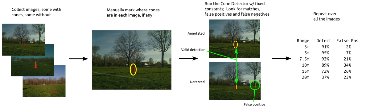
What we did in 2012, during the preparation for our first RoboMagellan, was take a lot of pictures of cones during our practice runs. Savage Solder normally is configured to save an image twice a second all the time it is running. These image datasets formed the basis of our ability to tune parameters and develop algorithms that would be robust in a wide range of conditions.
The basic idea we worked off was to create a metric for how good the system is, and then evaluate the metric over a set of data using our current algorithms and constants. You can then easily tweak the constants and algorithms as much as you want without running the car one bit and have good confidence that the results will be applicable to actual live runs.
Annotation Pipeline
Most of the metrics we wanted involved knowing where the cones actually were in the images. If we could just robustly identify cones in images programmatically, we wouldn’t really be worrying about this to begin with. So instead, we created a set of tools that let us rapidly mark, or annotate, images to indicate where the absolute ground truth of cones could be found. This is just a simple custom OpenCV program with some keyboard shortcuts that let us classify the cones in about 3000 images in a couple of hours. We selected images from varying times of day, angles, and lighting conditions, so that we would have a robust training set.
OpenCV Application for Annotation
Then, with a little wrapper script, we ran our cone detection algorithm over each of the frames. As mentioned in the on the cone detector, it outputs one or more range/bearing pairs to each of the prospective cones in the image. The quality metric then scores the cone detector based on accuracy of bearing and range to real cones, missed detections, and false detections. It also keeps histograms of each detection category by range. In the end, for a given set of cone detector parameters, we end up with a table that looks like the one below.
Range
Detection Rate
False Positive Rate
3m
91%
2%
5m
95%
7%
7.5m
93%
21%
10m
89%
34%
15m
72%
26%
20m
37%
23%
After each run over all the images, we would try changing the parameters to the cone detector, then seeing what the resultant table would like. Ideally, you have a much higher detection rate than false positive rate over the ranges you care about. The table above is actually the final one we were able to achieve for 2012, which allowed us to reliably sense cones at 15 meters of range using just our 640x480 stock webcam.
We got our final day of testing in at Danehy park in preparation for Robogames 2013 this weekend. Everything worked as well as we expected, the only things that would have caused problems on race day were trying to fit through areas too narrow for the basic GPS we were getting at the time. All in all, our speed, cornering, and tracking performance are much improved over 2012.
Along with many others, we’re hoping to enter our car into the Sparkfun AVC 2013 this year! In support of our effort, I put together some datasets and 3D assets that might be useful to other participating teams, especially if they do any work in simulation.
Georeferenced Data
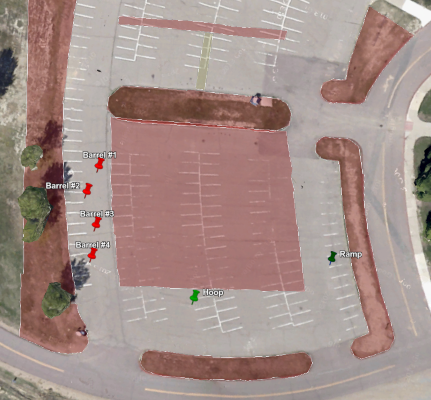
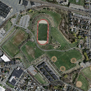
First, I used the most recent measurements from April 9th on the AVC website to create a kml file showing where each of the obstacles is, along with the course boundaries. I’ve included a snapshot from Google Earth below to show what it contains.
Sparkfun AVC 2013 Course Layout
Next, I extracted some freely available USGS ortho imagery and created a cropped version covering just the course. I essentially used the techniques described in my post on LIDAR imagery, except that the ortho imagery came from the USGS National Map Viewer. I created both a geotiff that has georeferencing information, and an opaque .png which is projected identically, but has no embedded information. On that last image, I did a little gimp hackery to edit out cars which would be in the path of the actual course.
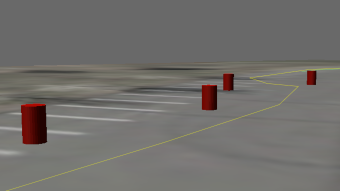
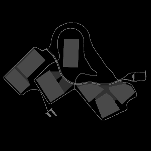
I also made a set of somewhat (OK very) crude blender models of each of the different obstacles present on the course to approximately correct dimensions. This includes the barrels, the hoop, and the ramp.
avc2013-barrel.blend
avc2013-hoop.blend
avc2013-ramp.blend
Drivethrough Video
Finally, just for fun, I recorded a screencast of one of the first drivethroughs of Savage Solder on the simulated Sparkfun AVC Course. This was with just the bare minimum of changes from what we’ll use at RoboMagellan in Robogames in two weeks, so for now it was navigating purely by GPS and IMU. It drives through the hoop about one time in three, which is enough to catch a good video! As in my previous simulation videos, the yellow line is where the absolute surveyed GPS path is. The green line is where the car thinks the GPS path is at any moment, which will differ due to GPS error and heading error.
Last time I covered the techniques we use on Savage Solder to pick out orange traffic cones from webcam images in the “Cone Detector”. This time, I’ll look at the next stage in that pipeline, turning the range and bearing reported by the cone tracker into Cartesian coordinate estimates of where any given cone is.
Cone Tracker Overview
As mentioned last time, our “Cone Tracker” takes as input the range and bearing, (along with their uncertainties), from the cone detector. It also receives the current navigation state of the car. This includes things like the current estimate of geodetic position (latitude and longitude), current map position, (UTM easting and northing), and an unreferenced local coordinate system (x, y). For each of these, it reports the vehicle’s speed and heading.
I won’t go into the details of each of these coordinate systems here, but since the cone tracker actually only uses the local one, I can discuss it a bit. The local coordinate system on Savage Solder starts out at x,y=(0m,0m) with a heading of 0 degrees at the beginning of every run. As time progresses, the heading and position are updated primarily based on our onboard dead reckoning sensors. The local coordinate system is smooth, and never jumps for GPS updates. As a consequence, it isn’t really useful to compare positions in it from more than a minute or two apart, nor is it useful to do GPS based navigation. Fortunately, for cone tracking, from the time to when we see the cone to when we touch it is usually only a couple of seconds total over which time the local solution is very accurate.
Now, let’s cover some broad details of the implementation. The guts of our cone tracker consists of a bank of identical Kalman Filters. Each Kalman filter estimates the position of one particular cone and the error in that estimate. This lets the car keep around several possible cones that could be in sight at one time while still distinguishing them. By storing the cones in a local coordinate system, it allows for easy driving towards, or alongside, the cone and accurate speed control leading up to it. The position uncertainty could be used to control behavior, but we don’t bother in our current implementation.
Cone Tracker Internals
New and Old Cones
Additionally, the tracker has to handle seeing new cones for the first time, and discarding cones that maybe were false detections in the cone detector. It does this by assigning each cone a “likelihood”, which is just a probability that the cone is a true detection. When data arrives that match the cone well, its likelihood is increased. When the available data doesn’t match the cone very well, or no cone is observed at all when one is expected, the likelihood is decreased.
If a range and bearing arrive which corresponds to no known cones, a new one is created with a relatively low likelihood. Then once it has reached a certain threshold, it is reported to the outside world as a valid target. Conversely, when an existing cone’s likelihood reaches a level which is too low, it is removed entirely on the thesis that it was actually a false detection to begin with.
More specifically, the likelihood update is handled using Bayes theorem. We have an empirically derived table showing, for our detector, the odds that a cone will be detected or a false one will be seen at various ranges. These are used to fill in the various probabilities in the equations.
Incorporating New Measurements
A “measurement” in this problem is simply the range and bearing that the cone detector reports. To incorporate a new measurement, the tracker looks through all the cones currently in its filter bank. For each, it computes a measure of the likelihood that the given cone could produce the current measurement. This is done using what’s called the Mahalanobis distance. The Mahalanobis distance is just a measure of how far away you are from an uncertain target in a multi-dimensional space.
If the best matching cone has a Mahalanobis distance small enough to count as valid, then the standard Kalman filter update equation is applied to that cone. If no cones match, then we create a new one as described above.
Scale Factor
Cone Tracker Flowchart
One final detail, is that in addition to estimating the position of each cone, the tracker also estimates its “scale” as seen by the cone detector. The image based detector we use has the property that the range values are likely to have a fixed scale error for a number of reasons. One, the cones could actually be bigger or smaller than the regulation sized ones. Second, lighting conditions can sometimes cause a fraction of the cone to be not detected, which will result in the cone being seen as smaller than it actually is.
Since the range values are not correct, the position will be similarly off. This error isn’t as bad as it seems, since we (and most every RoboMagellan entrant), approach the cone in a straight line. Thus the position errors will always be directly towards or away from the robot, and as long as you keep moving, you’ll hit it eventually.
Savage Solder has two reasons to care. First, is that we decelerate from a high speed to an appropriate “bumping” speed with just a half meter to spare. Thus, if the cone is estimated as too close, we run the risk of colliding with it at an unsafe speed and damaging our front end. Secondly, we have a mode where the car can just “clip” the cone by driving alongside it and tapping it with a protruding stick. This allows us to avoid stopping entirely when the geometry allows it. However, if the position estimate is incorrect here, we might miss the cone entirely.
Final Process
To summarize, the cone tracker handles each new range and bearing with the following steps:
A cone detection results in a new range, bearing, and uncertainty measurement.
Existing cones in the Kalman filter bank are checked to see what the likelihood is each could have produced this measurement.
If one was likely enough, then:
The position and scale factor are updated using the Kalman filter equations.
The likelihood estimate is updated according to our current false positive and false negative estimates.
If none was likely enough, then a new cone is created with a position fixed at the exact position implied by the local navigation solution and the range and bearing.
Any cones which we had expected to see but didn’t have their likelihood decreased.
Any cones which have too low of a likelihood are removed.
Finally, all the cones which are close to the vehicle, and have a high enough likelihood are reported to the high level logic.
Caveats and Next Steps
One of the challenges with this approach is that there are a lot of constants to tune. I’ll cover the details in a later post, but for most of them we tried to find some way to empirically measure reasonable values for our application. Another problem was debugging. printf doesn’t cut it when you have this much geometry. For that, we created a number of custom debugging and visualization tools which help show what is going on in the system, some of which I’ll cover later too.
One of the key aspects of our Savage Solder robomagellan solution is the ability to identify and track the orange traffic cones that serve as goal and bonus targets. Our approach to this is divided up into two parts, the first identification, the second tracking. They are roughly linked together with the block diagram to the right. Raw camera imagery is fed to the identification algorithm, which produces putative cones denoted by the bearing and range where they are estimated in the camera field of fiew. The tracking algorithm then takes those range and bearing estimates, along with the current navigation solution, and fuses them into a set of cartesian coordinate cones in the current neighborhood. Those local coordinates are then fed to the higher level race logic, which can decide to target or clip a cone if it is at the appropriate place in the script.
In this post, I’ll cover the Cone Identification Algorithm, listing out the individual steps within it.
Cone Detection Dataflow
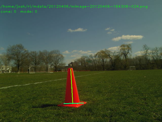
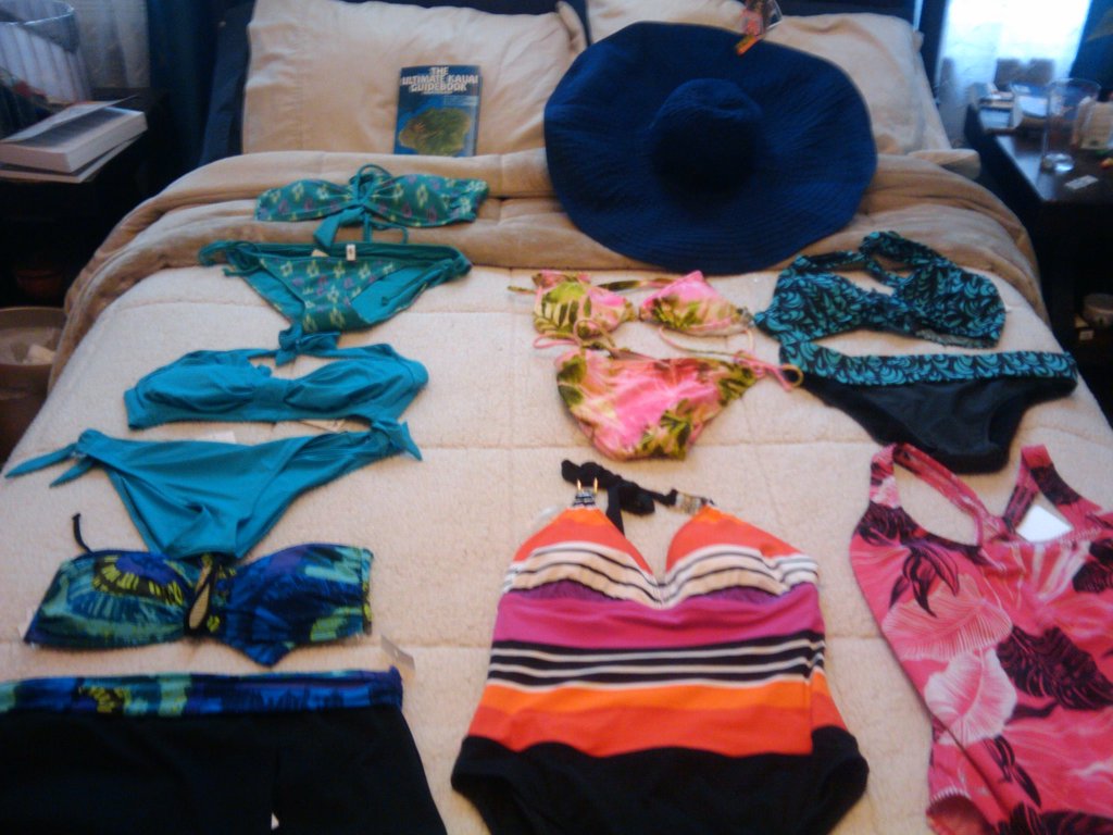
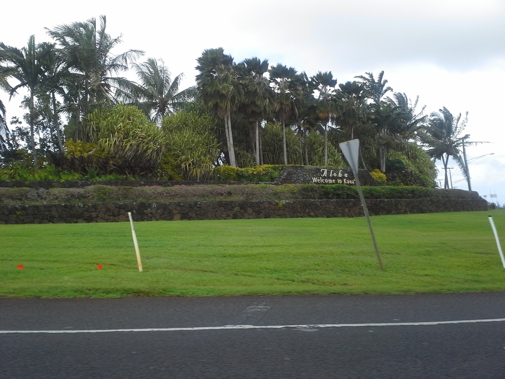
Original Image from Webcam
Our identification algorithm consists of a relatively simple image processing pipeline described below. We will work through a sample image starting from the source shown to the right:
Step A: First, we convert the image into the Hue Saturation Value color space, from the RGB values that our camera data source provides. In the HSV space, hue corresponds to color, and saturation and value determine how much color there is, and how white the color is. Since the traffic cones have a known color (orange), this helps us in later steps reject a lot of very unlikely regions of the visual field.
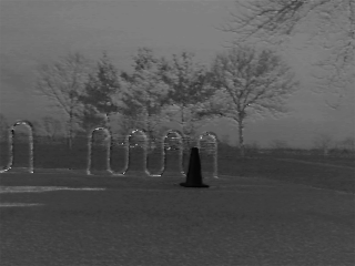
Hue Channel of HSV Transform
Step B: Second, we apply a limit filter to select only a subset of the hues and saturations, ignoring the value channel entirely. Both hue and saturation are parameterized by a center point and a range on either side of that center point which will be accepted. Since the hue values wrap around at 0, (red), we take care to select values on both sides of the center point. If the hue range does wrap around, we just do two limit operations, one for each side and merge the two together after the fact. The result of this process is a two color bitmap. It is black if there was no cone detected, white if there was a potential cone.
Bitmap with specific hue range selected
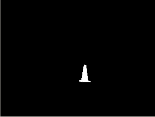
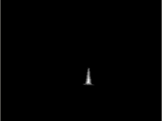
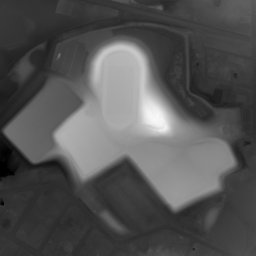
Step C: Next, we perform what OpenCV calls a “distance” transform on the resulting bitmap. This determines, for any given white pixel, how far it is to the nearest black pixel in any direction. Effectively, this will tell us how big any matched section is. It is not a terribly reliable indicator, as even a single black pixel in the middle of an otherwise large white area can result in halving the distance for all the pixels in that region. However, we use this to just discard regions that have a distance of 2 or less, which mostly throws away speckle noise. We also process each region in order of its distance score, so that we handle the biggest regions first.
Distance metric
Step D: At this point, we iterate through the connected regions starting at those which contain the largest “distance” points. For each, we measure the bounding rectangle of the region, and from that caculate the aspect ratio and the fill percentage of the region. The aspect ratio is just the width divided by the height. The fill percentage is the percentage of pixels inside the bounding rectangle which were marked as being a cone. To be considered a valid cone, the aspect ratio and fill percentage must be within certain configured limits.
Step E: Finally, if the putative cone passed all the above checks, the bounding rectangle is used to estimate the bearing and distance. The bearing estimation is relatively straightforward. We assume our camera has no distortion and a field of view of 66 degrees. From there, the x coordinate of the bounding box center linearly relates to the bearing angle. Range is estimated using the total number of pixels detected in this region assuming the cone is a perfect sphere. We calibrated the size of the sphere to match the visible surface area of a cone. If the detected region abuts one of the edges of the camera image, then range is not emitted at all, as the range will be suspect due to some of the pixels being off screen. The very last step is to estimate the bearing and range uncertainty, which the detector generates for 1 standard deviation away from the mean. A guess for the bearing value is made assuming a fixed number of pixels of error in the x direction. For range, we assume that some percentage of the pixels will be missed, which would errnoneously make the cone seem farther away than it actually is.
Next Steps
One all the qualifying regions are processed, or the maximum number of visible cones are found (4 for our case), then we call this image done and record the outputs. Next, these values go on to the “cone tracker”, which generates Cartesian coordinate positions for each cone. I’ll discuss that module later.
Earlier, we looked at how I used publicly available map data to create a simulation environment for Savage Solder, our robomagellan entry. Here, I’ll describe the process I used to source and manipulate the public GIS data into a form our simulation environment could use. There are two halves to this: the visible light imagery, and the elevation data used to build the 3D model.
Aerial Imagery
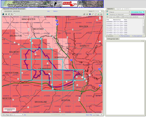
I started at the MASS GIS website located at: www.mass.gov. For Cambridge, that comes up with a tile map showing which tile corresponds to which area. From there, you can download MrSID data for the areas of interest.
MASS GIS Aerial Tile Map
The only free application I could find which adequately manipulated MrSID files was LizardTech’s GeoViewer, available for Windows only. I was able to use it to export a geotiff file containing the areas of interest.
Next, I used some tools from the GDAL open source software suite to manipulate the imagery (ubuntu package “gdal-bin”). The first was “gdalwarp”, which I used to do a preliminary projection into the Universal Transverse Mercator (UTM) projection. All of our vehicle and simulation software operates in this grid projection for simplicities sake.
The next step was a little finicky. I used “listgeo” (from ubuntu “geotiff-bin”), to determine the UTM bounding coordinates of the image. Then I selected a new bounding area which, at the same pixel size, would result in an image with a power of two number of pixels in each direction. Then, I used “gdalwarp” to perform the final projection with those bounds.
Where the UTM bounds are the same ones used for reprojecting the aerial imagery. Our simulation environment requires a terrain map be sized to an even power of 2 plus 1, so here 1025 is chosen.
Finally, this tif file (which is still in floating point format), can be converted to a discrete .png using gdal_translate. I use “tifffile” from the ubuntu package “tifffile” to determine the minimum and maximum elevation to capture as much dynamic range as possible. In this case, the elevations run from about 0m above sea level to 50m.
Last time working with the racing helicopter’s camera system, I managed to capture a poor quality image from the camera. My next step was attempting to diagnose the problems with the image quality. However, before I could do so, I ran into another problem with signal integrity in my breadboard setup.
The TI DM3730’s ISP with the 3.6 kernel is relatively sensitive to the quality of the pixel clock and vertical sync. If a single frame has the wrong number of pixels detected, the driver does not seem to be able to recover. This was a big problem for me, as the breadboard setup I have runs many of the 12MHz signal lines over 24 gauge wire springing around a breadboard. What I found was that I was only intermittently able to get the ISP to capture data, and eventually it got to a point where I could not get a single frame to capture despite all the wiggling I could attempt.
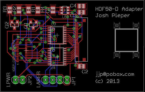
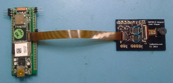
Rather than spending a large amount of time trying to tie up my breadboard wires just so, I instead just printed up a simple adapter board which contains all the level translation and keeps the signal paths short. This time, I tried printing it at oshpark.com, a competitor to batchpcb. The OV9650’s FFC connector has pads with a 7.8mil spacing, and batchpcb only supports 8.1mil, while oshpark has 6mil design rules. They also claim to ship faster, and are slightly cheaper.
The results were pretty good. From start to finish, it took 14 days to arrive, and the 3 boards appeared to have no major defects. My art had one minor error which required rework. The output enable pin on the level converters were tied to the wrong polarity, thus the lifted pins and blue wiring. Despite that, it appears to be working as intended.
For our simulation environment, we currently rely on digital elevation maps from the city of Cambridge along with aerial imagery of the environment. The simulator places the car in that fake world, and pretends to be each of the sensors that the car has. For Savage Solder, that is the IMU, the GPS, and the video camera.
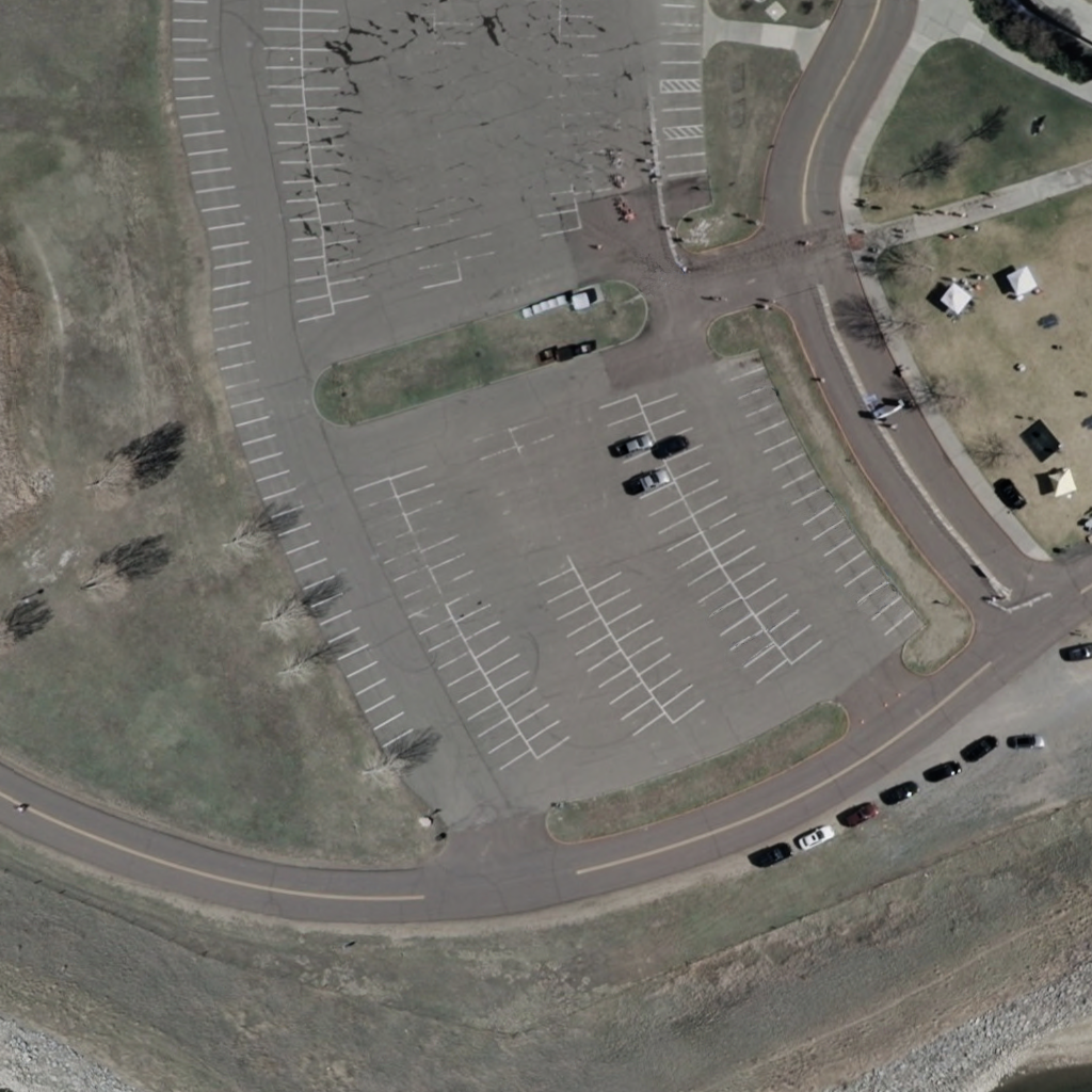
In this first stage of staying on the pavement, we added an additional “oracle” sensor which has roughly the same field of view as the camera, but instead of reporting images, reports how fast the car can go at any point visible in the frame. The simulator gets this information from a hand-annotated map of the test area, where each pixel value corresponds to the maximum allowed speed. For example, below is downsampled aerial imagery of Danehy park in Cambridge, along with the hand annotated maximum speed map.
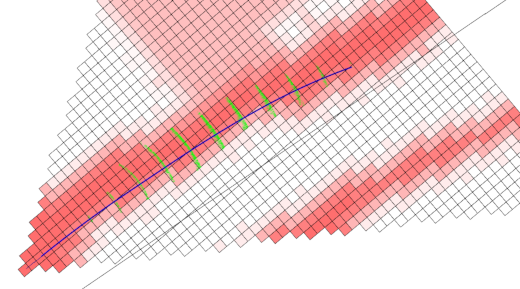
The locally referenced terrain data is fed into the online replanner. Currently, the maximum speed is just used as a penalty function, so that the car prefers to driver over terrain labeled with higher speeds. A sample online replanner output is shown below. Here, darker shades of red imply a higher maximum speed, and the black line is where the global GPS waypoints are in the current local reference frame. You can see the planned trajectory follow the red path despite it being offset some distance from the global trajectory. In practice, this will happen all the time, if nothing else because the GPS receiver on Savage Solder is comparatively low accuracy and often drifts by 3 or 4 meters in any direction.
Online replanning on a sidewalk
As a caveat, the implementation now actually still drives at the speed programmed in by the global waypoints regardless of what the local maximum speeds are. The local sensor just modifies where it drives. Fixing that up is the immediate next step.
We hope this approach to also be useful for events like the Sparkfun AVC, where the traversable path is of the same size or narrower than the GPS accuracy.
 avc2013-barrel.blend
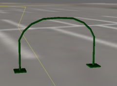 avc2013-hoop.blend
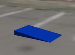 avc2013-ramp.blend
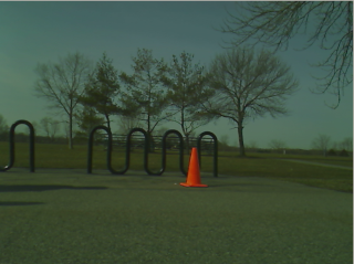


