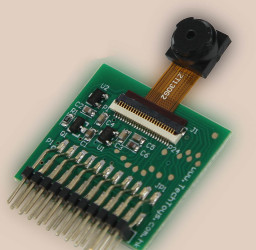
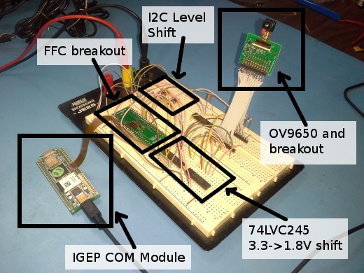
In my previous post I described how I wired up an OV9650 based camera module to my IGEP COM Module. The ultimate goal of course is a low cost reliable altimeter for my autonomous racing helicopter. When we left off, I had the camera breadboarded up connected to the IGEP COM Module and wanted to drive it over the I2C interface to verify it was working. While the IGEP COM Module’s camera I2C interface is easily exposed to the linux user space, the OV9650 doesn’t respond to I2C commands without a clock being present. Turning on the clock turned out to be quite a challenge.

First I explored the possibility of existing user space tools which might be able to poke directly into /dev/mem and activate the clock. Promisingly, I found omapconf, a user space tool which claimed to provide complete control over the clock systems of TI’s OMAP chips. Unfortunately, it only operated on OMAP4 and the unreleased OMAP5, not the OMAP3 that is in the IGEP COM Module. The source code wasn’t particularly helpful for quick inspection either. There is a lot of complexity in manipulating the processor’s clock registers, and implementing it from the datasheet didn’t seem like a particularly fruitful use of time. Thus discouraged, I moved on to the next possibility, kernel mode operations.

The linux kernel for the IGEP COM Module already had routines designed to manipulate the clock registers, so why not use those? Well, to start with, building a custom kernel (and suitable system image), for this board was hardly well documented. After much consternation, and then much patience, I ended up piecing together a build setup from various IGEP wiki pages that allowed me to mostly reproduce the image that came on my board. It consisted of the following steps:

• Yocto: Is a tool used to creating embedded linux distributions. It is based on the OpenEmbeddeded recipe files, and includes reference layers for building a distribution.

  git clone -b denzil git://git.yoctoproject.org/poky
  

• ISEE Layer: ISEE publishes a yocto layer for their boards which includes recipes for a few packages that don’t yet exist in yocto.

  git clone -b denzil git://git.isee.biz/pub/scm/meta-isee.git
  

Once the relevant git trees were cloned, you still have to generate a build/directory using the “oe-init-build-env” script, and modify files in that directory to configure the build. The How to get the Poky Linux distribution wiki page on the ISEE website had some hints there as well.

With this configured, I was able to get a system image that closely matched the one that came with my board. In addition, I added a local layer to hold my modifications, then proceeded to switch to the as yet unrelease ISEE 3.6 kernel, which has support for the ISEE camera board. My supposition is that the OV9650 camera I’m working with is close enough to the mt9v034 on the CAM BIRD that I will run into many fewer problems using their kernel. For my local development, I cloned the ISEE kernel repository, and have pointed my local layer’s linux kernel recipe to the local git repository. This allows me to build local images with a custom patched kernel. Now, I am truly able to move on to the next step, of driving the clock!

What I expected to be the hardest hardware portion of the ARR has not disappointed – the camera. To recap, I am in the process of designing and building an autonomous helicopter. As part of that, I wanted to use a vision system combined with a laser pointer to provide low cost altimetry during takeoff and landing. The IGEP COM Module has a dedicated camera port with support for both camera and serial interfaces, and there are a large number of cheap camera phone camera modules out there which should be sufficient. How hard can it be?

I started with a TCM8230MD from SparkFun for which I simultaneously ordered a breakout board from some random online retailer. Unfortunately, the breakout board never came. I tried using some 26 guage wire I had around and a magnifying glass to solder up a by-hand breakout board to no avail. Finally, I broke down and found http://sigalrm.blogspot.com/2011/03/tcm8230md-breakout.html who posted eagle files of a breakout board. I dutifully submitted them to batchpcb and waited.

While I was waiting for batchpcb, I simultaneously ordered an OV9650 based board from techtoys, who also sold a breakout (pictured right). While the breakout was on 1mm spacing instead of 0.1in spacing, it was still a lot easier to experiment with. The Hong Kong post has gotten remarkably good, because this development board arrived long before the batchpcb breakout did, so I started integrating it. This board operates at 3.3V, while the TI DM3730 in the IGEP COM Pro uses 1.8V for all of its external IO. To mediate between them for logic level signals, I used a bank of SN74LVC245ANs from digikey, along with 2 discrete N-FETs to shift the I2C bidirectional signals as described in this application note from NXP.

The next challenging step was getting the camera port on the IGEP COM Pro into a usable form. It has a 27 pin 0.3mm FFC style connector, which if you haven’t seen one before is tiny! To make this work, I got a 4 inch passthrough cable from digikey and mating connector, and this 0.3mm FFC breakout from proto-advantage.com. I soldered down the FFC connector to the breakout using my hot air rework station, but should have used an iron with solder-wick technique, as the plastic on the connector melted and bubbled up a bit during soldering. Fortunately, it still worked, so I didn’t need to use my spare.

At this point, I had the camera and IGEP COM Module nominally wired up in a way that should be usable. The final breadboard is pictured above. To make progress from here, I wanted to try a smoke test: communicate with the camera over it’s I2C interface to verify that it is powered and working. However, I quickly discovered that it wouldn’t do anything unless it was supplied with a valid clock. This turned into my next odyssey – trying to enable the clock output on the TI DM3730 in the IGEP COM Module. That is involved enough to be the subject of a later post.

This is a followup to my last post discussing the initial platform controller feasibility experiments for the ARR, my autonomous helicopter.

We left off last time with a couple of candidate designs for the platform controller and some rough requirements that it needed to meet. What I wanted to do was devise a test procedure that could ensure that it would meet all the functional, as well as performance requirements, preferably over a long period of time.

Basic Functionality Testing

First, the controller has a moderate number of relatively performance insensitive functionality that could potentially regress. This includes things like reading GPIO inputs, configuring what inputs to stream, and communicating over the I2C bus. For these, I created a pyunit test suite communicating with the device over it’s USB-serial interace with pyserial. The suite setup function forces the platform controller to reset, so each case starts from a known state. From there, I created maybe a dozen tests which exercise each piece of functionality and verify that it works as expected.

Input Servo Pattern Generation

Next, the platform controller needs to be able to sample 8 servo channels with sub microsecond precision. To verify this, I needed to generate 8 channels of data which were both a) easily verifiable as correct, and b) likely to turn up most of the likely causes of performance problems. My eventual solution was to create a very simple AVR program running on a separate microcontroller using delay loops which emits 8 channels of servo data with pseudorandom values using a known linear feedback shift register (LFSR) equation. I used a 16 bit LFSR, emitting only the upper 11 bits as the pulse width. Each channel was exactly one LFSR cycle behind the previous one in time, so that for a given 8 pulse cycle, you will have seen 8 subsequent values of the LFSR. This made it pretty easy for the receiver to figure out what the remaining 5 bits should have been, even if there were errors of several LSB (least significant bit) on several of the channels. For example, a few cycles of this pseudo-random data look like:

#        Channel pulse width in hex.
# Cycle   1   2   3   4   5   6   7   8
   1     370 1B8 0DC 46E 237 11B 48D 246
   2     1B8 0DC 46E 237 11B 48D 246 123
   3     0DC 46E 237 11B 48D 246 123 491

This approach has a couple of benefits:

• Each 50Hz cycle is independently verifiable. All you need to do is scan through all possible “hidden” 5 bits and see if any result in a close match across all channels. You can also see just how much error there is on each channel.
• Every channel changes drastically at each cycle. Some problems could be masked by slowly time varying inputs. Since at each cycle, the input changes in a very random way, this isn’t a problem.
• The emitter can run open loop. No test harness communication is needed with the servo control emitter whatsoever. It just emits the random 8 channels of servo data indefinitely.

I wired up this separate AVR to the platform controller on a breadboard, and first added a few simple tests to the pyunit test suite that checked just a couple cycles to verify basic consistency. Once that was working, an endurance test script streamed the input data (along with a representative sample of other data as well to simulate comparable load to the final system), checking each frame for consistency and the number of LSB errors.

Servo Output Performance

The ARR platform controller has the ability to either pass through servo inputs, or take commands over the USB-serial link. Both of these needed to be verified in a comprehensive way. Fortunately, after the input verification step above, I already had a microcontroller which could sample 8 servo channels with high accuracy and report them back over a serial link! So I solved this by just dropping another ARR platform controller onto my breadboard. The pyunit test suite was extended to communicate with both devices, and monitored the outputs of the device under test using the second system. The final test harness block diagram is below:

Overall System Performance

Using this complete system, the endurance test script verifies not only input performance over time, but output performance over time as well. In one sample run, I got the following results:

 Frames capture: 150,000 (about 50 minutes)
 Input Results:
   Invalid Frames:       0      - 0.00%
   Values w/ 1 LSB off:  5,601  - 0.47%
   Skipped Frames:       0      - 0.00%
 Output Results:
   Invalid Frames:       0      - 0.00%
   Values w/ 1 LSB off:  58,000 - 4.82%
   Skipped Frames:       0      - 0.00%

These results were taken when the platform controller was passing through input values to the output and streaming a full complement of I2C data at 100Hz. They are about as expected, a single servo value results in a 1LSB error about 0.47% of the time. Then, passing that channel through to the output and sampling it a second time results in a 1LSB error about 4.82% of the time. Given that 1LSB of error will not even be noticeable in this application, these results are just fine. Finally, for posterity, I’ve included an annotated picture of the completed test harness below:

For my nieces this holiday season, in addition to actual cookies, I printed up some customized cookie cutters on the Artisan’s Asylum 3D printer (A Stratasys uPrint SE Plus)

Inkscape

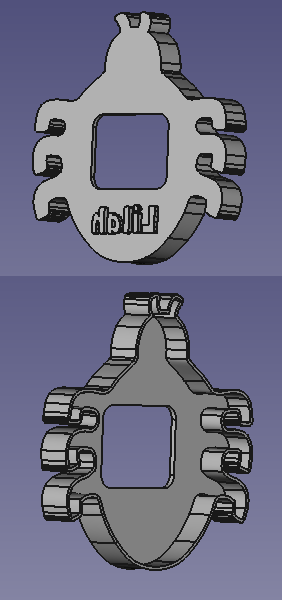
The toolchain I used could be applied to a number of 3D projects. First, I either found an image kind of resembling what I had in mind using google images, or drew up a sketch on a piece of paper. Then, I transcribed that image into an inkscape vector drawing, similar to the elf one on the right. The inkscape drawing contained a closed shape for the outer dimensions of the part, the inner dimensions of the part, as well as closed shapes for any surface features that I wanted. I used the “Linked Offsets” feature to force the inner wall boundary to be a precise distance away from the outer wall boundary. Colors were chosen arbitrarily, as the next step ignores the fill colors entirely.

Freecad

Next, I fired up freecad, which can import SVG elements as geometry primitives in the 3D view. Unfortunately, and what was to become the biggest annoyance with this project, is that its import of SVG paths isn’t particularly robust. Notably, for some elements it doesn’t close them properly, and for others it doesn’t even turn them into curves, rather importing them as sets of points. This was done in a hurry, and while I didn’t have enough time to actually fix the problems in freecad, I did dig around in the source enough to figure out that they were not handling paths which ended up on the exact same position as the first point correctly. One problem was that freecad would only count a path as closed if the “z” element was used to close it off. Another was that paths with kinks would just not close with no indication why, even if the kinks were too small to be visible. So, my workaround was to manually edit the .svg files in emacs after inkscape saved them and fiddle around with them afterwords to try and get freecad to import them as closed surfaces. Then for the paths that still didn’t work, I looked extra close in inkscape for any kinked paths. In this project, those largely resulted from inkscape’s linked offset paths being glitchy around regions of high curvature.

With those surfaces imported, I then proceeeded to do a series of extrusions, differences, and unions to get the parts that I was looking for. In some cases, when I ran into limitations of freecad’s boolean operation engine, I had to go back to inkscape to tweak the artwork. This was largely around different objects which were intended to share a border, which didn’t work out so well.

netfabb

After getting the solid models into good shape in freecad, I exported an .STL file for each model. I pulled this .STL file into netfabb studio basic to verify the volume and to do mesh repair. Sometimes freecad will export .STL files that netfabb doesn’t complain about, but I figure it doesn’t hurt to let it fix up any problems it finds.

uPrint 3D Printer

The final step is printing. This is largely uneventful: feed in the STL files, configure the print job, hit print, and come back in a couple of hours. Usually, when printing a part, you can count on the first iteration to have some problems and this case was no exception. I had designed the cookie cutter wall thickness to be 1.25mm wide, figuring that would be 5 passes of the uPrint. However, the uPrint ended up not actually filling the inside of the wall in many places, resulting in two very thin walls separated by a small void. Given more time, but in this case I was out, so I moved onward with what I had!

Baking!

So, the final test, using them to cut cookies… Well… They mostly worked. The separated outer walls caused a lot of cookie material to get wedged up inside. I also realized at this point why most cookie cutters have an exposed central area. Without one, extracting the cookies is quite challenging. I painstakingly used chopsticks and a knife, which worked adequately, if with great effort. Certainly, if I were to make a second revision, I would fix both the separated wall problem, and make the cookies easier to eject afterwards.

Below is a picture of the final 3 parts before being gummed up with a season’s worth of cookie making.

The first aspect of my autonomous helicopter project I tackled was to validate the feasibility of an AVR microcontroller based low level platform controller (more specifically, the AT90USB1286). The platform controller needs to provide the real time interface between the radio receiver, the servos, the primary flight computer, as well as a couple of additional sensors. More specifically, the platform controller has a couple of responsibilities and/or requirements:

• Receive up to 8 channels of servo commands from the radio receiver.
• Emit up to 8 channels of servo commands to the various servos and motors on the helicopter.
• Optionally allow the receiver commands to pass through to the output, or alternately put the outputs under computer control.
• Communicate with a variety of I2C devices, notably the inertial sensors and a barometer.
• Expose all of these sensors to the flight computer over a full speed USB connection.

A block diagram showing the interconnections in the current design is below

The servo command manipulation is particularly challenging. As a refresher, most RC servos are controlled with a pulse width modulated signal, where a pulse of between 1ms and 2ms is emitted at 50Hz. 1.5ms commands the center position and the other two extremes are at 1ms and 2ms. The Spektrum receiver on my Blade 450 claims to have 2048 bits of resolution. That indicates that each least significant bit (LSB) of command corresponds to (2ms - 1ms) / 2048 = 488ns. Given that most AVRs have a maximum clock rate of 20MHz, that works out to about 9 AVR clock cycles per LSB. In general, sampling an input with that level of accuracy would require a hardware capture register, but no AVRs have 8 separate inputs which can trigger captures.

Input Approach 1: Analog Comparator and Timer1 Capture

I explored two mechanisms for getting around that shortcoming. First, while the AVR does not have 8 separate inputs which can simultaneously be connected to a capture register, it can be configured to allow the analog comparator to trigger captures. Subsequently, the analog comparator can be driven by the analog multiplexer, which on the AT90USB conveniently has 8 inputs. The downside is that only one input can be selected at a time. This isn’t necessarily a showstopper, as most RC receivers actually drive the servo commands one after another in time. Channel 1 is pulsed, then channel 2, channel 3, and so on. Then when the time for another 50Hz cycle begins, the cycle starts afresh.

My experiments with this approach were mixed. The accuracy was very good, since the capture was done by the AVR hardware, I could accurately sample at 20MHz when each pulse started and stopped. There were downsides though. For one, the receiver servo outputs had to be connected in exactly the correct order. If they weren’t, then the wrong pin would be configured when it was being pulsed. While the pin orderings will be fixed in this application, the firmware may be useful in a more general sense later. The need to whip out a scope to find out which order the pulses are emitted in could be a little burdensome. Second, and more critically, all of the processing for this approach was done in a main loop, including switching which input pin was being sampled. This was done to minimize the amount of time with interrupts disabled in order to support accurate servo pulse outputs. Because of this, occasionally the main loop would not complete a full cycle between when pulse N stopped, and pulse N+1 started, and the pulse would be missed, along with the rest of the pulses that cycle. Similarly, it requires that disconnected channels be placed altogether at the end. While these limitations may not be showstoppers, I wanted to see if I could do better.

Input Approach 2: Pin Change Interrupt

The second approach was to sample the servo inputs by placing them on the AVR’s 8 bit pin change interrupt port and configuring that interrupt. Then, the interrupt handler samples the current value of a timer, enables interrupts, then samples the state of the input port. Both values are stored into a ring buffer for consumption by the main loop. This approach requires about 16 instructions to execute in the interrupt handler before interrupts are re-enabled, which could introduce ~1 LSB of jitter into the output pulses if the timing is unfortunate. However, it can handle servos connected in any order and can handle any input being disconnected. This approach seemed relatively promising, my experiments proved it out with roughly the above properties.

Servo Outputs

Next, the AVR needed to generate the 8 channels of output in an accurate way. The technique that ended up working well for me was to, in the main loop, start a servo pulse output and begin a countdown timer in a small critical section protected with interrupts disabled for 3 instructions total. Then, the interrupt handler is hand coded in the minimal amount of assembly to zero out all the outputs on the given port. gcc by default, if you write:

ISR(TIMER3_COMPA_VECT) {
  PORTC = 0x00;
}

Will generate 12 instructions of prologue and code to save the status, r0 and r1, xor r0 with itself to generate a 0, then store r0 to PORTC, and finally restore everything. What I ended up using was:

ISR(TIMER3_COMPA_vect, ISR_NAKED) {
  asm("push r16"     "\n\t"
      "ldi r16, 0"   "\n\t"
      "out %0, r16"  "\n\t"
      "pop r16"      "\n\t"
      "reti"         "\n\t" :: "M" (_SFR_IO_ADDR(PORTC)));
}

Notably, there is an AVR instruction to directly load an immediate into a register without affecting the status register, so it doesn’t need to be saved. Also, only one temporary register is required, whereas gcc prepares two for no good reason. This hand assembly requires a mere 5 instructions, significantly reducing jitter coupling into the input sampling loop.

Next Steps

Next time, I’ll look at how I stress tested this solution to verify that it would actually work over a long period of time and through all the required scenarios.

In part 1 and part 2 I looked at our progress in improving the acceleration performance of our Savage Solder autonomous racing car as applied to RoboMagellan type competitions. We left off with a reliable open loop model of acceleration versus current speed and throttle input, which were combined with some feedback elements to make a simple controller. However, upon running the controller the first time, we saw some odd behavior when the throttle transitioned to and from braking. It was difficult to see at our standard sampling rate of 20Hz, so we increased our overall control loop to 50Hz (the rate at which the RC servos are updated) to get a better view. The behavior can be seen on the plot below:

Around time 15:32:24.9, the throttle command switches from a braking command to a positive acceleration. Then just before 25.0, the velocity starts a rapid ramp up for 4 time samples, starting from about 1.4 m/s and peaking at about 2.0 m/s, a 40% increase. After those 4 samples, it snaps back into place at around the previous value of 1.4 m/s. This type of velocity spike occurs on nearly every transition between accelerating and braking.

What is happening here is caused by the backlash in the car’s transmission. There is a region of about 3-4cm where you can move the drive wheels without turning the motor caused by the aggregated slop in all the individual linkages between the motor and the drive wheel. The car is not actually speeding up or slowing down during this event, but the motor (where our velocity data comes from) does. It speeds up until all the backlash is consumed, at which point it then resumes traveling at the exact same speed as the rest of the car. This was confirmed by looking at auxiliary inertial measurement data which indicated that the car itself did not accelerate or decelerate during these events.

Once suitable filtering was in place to mitigate the effects of backlash, our velocity control is performing admirably on pavement test surfaces. Below is a plot of a demonstration run with a top speed of 15 mph, an acceleration of 3.0 m/s^2, and still decelerating in a controlled manner to bump a cone. With our current tuning, it starts decelerating about 8s before contacting the cone. We were just able to get enough space in our test area to get it to hold 15mph briefly. Note the accurate velocity tracking both during hard acceleration and deceleration, as well as the smooth approach into the final bumping speed.

And finally, video we took of the car when the above data was recorded:

 

In the previous installment, I looked at the problems we had with Savage Solder’s legacy PI velocity control loop when used for RoboMagellan type competitions. This time, I’ll look at how we measured the characteristics of the car, motor, and motor controller.

We wanted to get a better understanding of what the open loop behavior of the car was at a range of accelerations – and on a variety of surfaces. So, I fired up our primary application, which just happily logs data from all systems when the transmitter is in manual override mode. Then, I had a lot of fun driving around a bunch. Practically though, I tried to get instances of differing throttle values at as many different speeds as possible. So I tried to accelerate and decelerate at different rates as fast as I felt comfortable going in the space I had to drive. I repeated the process in some grass to get a feel for how the behavior differed there. Finally, I pulled all the data off the car and started the analysis.

My theory was that for a given terrain, speed, and throttle, the car would exhibit a particular amount of deceleration or acceleration. This assumes that the motor controller is stateless, but otherwise encompasses a range of possible motor controller implementations. At each instant in the data file, I measured the instantaneous acceleration by sampling the velocity some fractional time before and after. Then, I created a 2D grid defined by the possible car velocities and throttles, and for each grid cell accumulated the observed accelerations. This average acceleration for each cell was then plotted using matplotlib’s tricontour function. Below I have included a sample plot from pavement and grass driving.

Notably, this plot has no information about regions of braking action. It turns out that it was extremely hard to actuate a suitable range of braking actions from different speeds when driving by hand. Instead, we ended up running dedicated experiments where the car started from a steady state known throttle, then commanded a constant braking throttle until the car stopped. I repeated this for a range of braking values, starting from as high a speed as I was able to do in our back lot testing area. The below plot shows those values.

The data pretty much matched the hypothesis. In fact, the acceleration could be accurately modeled using a simple electric motor model where the throttle input directly controlled the voltage applied to the motor when powering forward. A similarly simple model matched the braking behavior. These models were enough to create a velocity controller which can accelerate and decelerate much faster, while still maintaining position accuracy of velocity. However, before we were able to make it work robustly, there was one other annoyance which I’ll discuss in the next post, motor backlash.

One of the areas of improvement we are working on for Savage Solder is velocity control. More specifically, we are improving the performance of the velocity controller at higher speeds and higher accelerations. In our runs during the spring of 2012, we had a simple PI controller on velocity let the car safely run around 5-7mph with accelerations around 0.7m/s^2. Given that the underlying platform can exceed speeds of 40mph and accelerations of 4m/s^2, we wanted to get a little closer to the theoretical maximum in order to reduce event times. Here, I’ll look at why the original controller was limited, and what properties we wanted an improved controller to have.

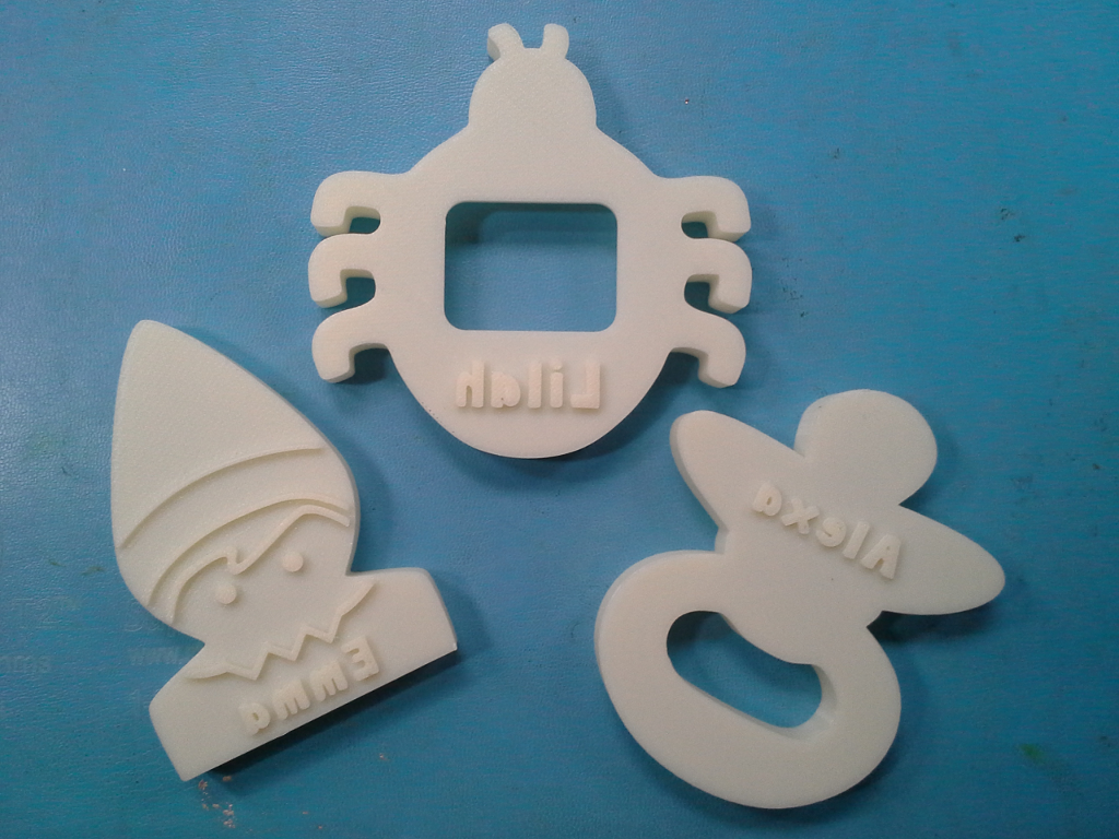
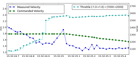
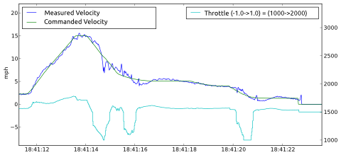
First, a little background. The motor controller on Savage Solder is the stock HPI Savage Flux controller, configured with a sensored brushless motor. For input, it uses a standard RC servo control pulse width signal from 1ms to 2ms in duration at 50Hz. We logically treat it as having a range of throttle command values of between -1.0 and 1.0. In forward motion, the default configuration has increasing positive values used to increase speed, and increasing negative values to apply braking forces. It can also move in reverse, but requires a small lockout window of stopped time, and in reverse, no braking is possible. Forward commands always result in attempting to move the wheels forward regardless of the current directin of motion. You can configure different behaviors, but these are the factory default and most of the alternatives involve removing reverse capability entirely, which we require. When driven manually, the throttle is very sensitive. Given the car’s very fast top speed, it takes very little movement on the throttle trigger to accelerate the car up to speeds that would require a wide open tarmac to navigate safely. Similarly, it takes some skill to not flip the car over end over end during both acceleration and deceleration. The figure at the right gives a simple representation of these properties. Note that the magnitude of the increasing speed and brake power is not specified and in fact the region near 0 throttle is also undefined.

The legacy velocity controller for Savage Solder was a simple PI controller, with a small state machine surrounding it to reset it and wait the required time upon switching from forward to reverse motion. In this formulation of a PI controller, the integrative term “finds” the appropriate throttle over time, while the proportional term improves the dynamic response by applying extra throttle based on the instantaneous error. Given a long time, and a constant speed command, this controller had no problem converging on that speed with precision. The plot below shows some data from the spring where the car accelerates up to 8 mph. You can see that the actual speed converges on 8mph in a second or so.

The problems with this solution became more apparent at higher accelerations. Since the integrative term requires error in order to equalize, the higher the acceleration, the larger the steady state error during the acceleration. This isn’t often much of a problem during cases of speeding up, but when slowing down it can be a big deal. Our approach for the Robo-Magellan competition (and most other entrants), involved bumping the target traffic cones at low speed. If the speed controller lags in deceleration by several seconds, the car would just plow over the cone rather than stop in front of it. The other major problem is during the transition from a regime of constant acceleration to one of constant speed, especially when slowing down. The integrative term can take a long time to wind back down, during which time the car is completely stopped. In the 2012 Robomagellan event, this was magnified by transitioning from pavement to tall grass right near the end of the deceleration into the first bonus cone. Finally, to mitigate these problems somewhat, we set the P gain to be larger than would otherwise be desirable. The result of this higher gain in the plot above can be seen as small oscillations in the speed and commanded throttle.

When designing an improved solution, we considered the two primary event types that we were planning to compete in:

• Robo-Magellan: As mentioned above, tracking accuracy on deceleration is a must, otherwise the car could overrun the targets. High acceleration and deceleration rates are useful too, as targets are often in close proximity, not leaving much room to speed up and slow down.
• Sparkfun AVC: In this event, deceleration accuracy is not as important, but top speed and acceleration are. You basically speed up once, and decelerate briefly for each of the 3 turns.

Next time I’ll look at the experimental path we took, and the next iteration of the velocity controller which we used to improve the performance.

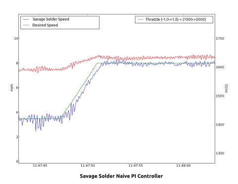
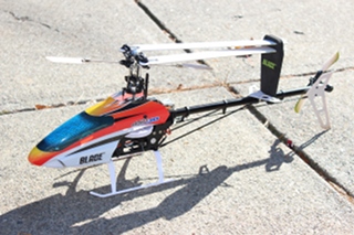
For the last 6 years I have ever so slowly been learning how to fly medium sized RC helicopters outdoors, in an attempt to become a good enough pilot that I could roboticize one. About a year ago I upgraded to a Blade 450, which let me practice outdoors in a much wider variety of weather conditions and provided for a feasible amount of payload. My proficiency is now good enough that I’ve started work on the control and navigation design with the medium term goal of entering it in autonomous racing competitions, such as Sparkfun’s AVC.

At the top end, this helicopter can lift around 100g, which while tight, should be completely doable with 2012 componentry. A rough outline of the components I have in mind now is:

• Computer - IGEP COM Module: A gumstix clone out of Spain, they are slightly smaller, slightly more powerful, and can nominally be powered and operated over USB with no baseboards required. (Although I’ve so far found that heat issues pretty much require a baseboard or other heatsink of some kind be used.)
• GPS -Sparkfun GS407: We had reasonably good luck with the u-blox 6 chipset on Savage Solder. It doesn’t have great precision, and has no way to bypass the internal EKF, but at least lets you configure it somewhat.
• IMU - Currently I’m planning on using the same chips as in the Pololu MinIMU-9 v2 just because I’ve worked with it on Savage Solder, the drift performance is reasonable, and the combined electronics only add a couple of grams.
• Altimeter - My hope is to use a structured light solution where a small camera-phone camera module looks down coupled with a laser pointer offset by some amount. The laser pointer will alternate one frame to the next to increase the signal to noise ratio. Then, the position of the pointer in the camera’s field of view should give a relatively accurate altimeter at ranges between 1 and 10m. Higher than that and I am figuring GPS will be good enough to keep it far from the ground.
• Servo Control and Failsafe - To develop the autonomous system with a minimum of crashes, it will need the ability to be controlled both by a human and by the computer, with an emergency fallback to human control. Also, for simulation modeling purposes, I want to be able to record the human inputs made during manual flights. In order to not require hard real-time performance of the linux-based IGEP board, I will use a separate AVR controller to read, pass through, or command each of the servo channels. The Blade 450 only has a 6 channel transmitter, (throttle, pitch, roll, collective, tail, and gyro gains). In case of an upgrade later on, I’ll assume that there are 8 transmitter channels that might need to be manipulated.

I have a preliminary set of milestones laid out. While each may end up taking significant effort, it will at least let me track progress. They don’t all necessarily need to be done in order of course:

• Demo Servo Control - Demonstrate that the AVR can monitor, passthrough, and command 8 servo channels while simultaneously reading full 100Hz updates from the I2C IMU, and feeding everything back over the USB link without losing accuracy. I have a working implementation of this, which I’ll cover in a later post.
• Camera and Lens Selected - Prototype and get a camera working with the IGEP COM Module and verify that its optical properties will be sufficient for altimetry and possibly horizontal motion compensation during landing.
• Block Diagram of Daughterboard - Draw up all the major components required for the daughterboard.
• Schematic of Daughterboard - Actually capture all the connections and minor components necessary for the daughterboard.
• Layout of Daughterboard - Get the first rev of the board drawn up and manufactured.
• Board Bringup - Get the board working, re-print as required.
• Flight Data Recording and Simulator - Using the flight hardware, take data of flights and use it to build a simulation model. Currently, CRRCsim looks like it will be suitable for a dynamics and visualization platform. It’s rotorcraft support isn’t great, but with some work I believe I can get it close enough.
• Navigation Filter - Using the simulator and flight tests, create a navigation solution which can accurately localize the helicopter in 6D.
• Autonomous Forward Flight - Fly simple autonomous trajectories in fast forward flight.
• Prove out Altimeter - With manual takeoff and landing, get the altimeter to a satisfactory level of performance.
• Autonomous Takeoff and Landing - Using the altimetry when close to the ground, make controlled landings and takeoffs.

Wow, that is a long road ahead.

Very belatedly reported, Mikhail and I entered Savage Solder in the Robogames 2012 RoboMagellan competition, placing first. The goal was largely to see what we could do in a short period of time. With only about 2 months from start to finish, we put together a machine which handily took first place in the competition, despite having a few significant bugs and barely having been tuned for performance.

The strategy was relatively straightforward: Start with a capable platform, we used the HPI Savage Flux with a laptop, webcam, GPS, and IMU strapped on top. A Teensy USB was coded to read RC servo inputs, write servo outputs, talk to the IMU over I2C, and read the bump sensor while connecting to the laptop over USB. A simple Unscented Kalman Filter (UKF) kept a global world position using GPS in UTM coordinate space. The car followed trajectories using pure pursuit for steering and a PID controller around velocity. The trajectories were layed out ahead of time with a simple lua script that pointed them towards each of the cones in a series using Dubin’s curves. A separate target tracker maintained UKFs for one or more visible cones which were culled from a simple visual filter. Once a cone was certain enough, and in the right location, the trajectory tracker switched to making trajectories aiming at the cones and slowing down, until a forward facing bump sensor tripped. At that point, the car moved on to the next element in its sequence.

The biggest thing we didn’t even include in our design was obstacle detection or avoidance. With the u-blox GPS we used, we were able to achieve positioning performance that would usually constrain the car to within +- 1.5m of a desired path, which, together with careful manual planning, was mostly enough to keep it from running into things. This was helped by the fact that the landscape for current RoboMagellan events is relatively forgiving, having few dynamic obstacles which aren’t people.

The two biggest failings in the design were that 1) we ran out of time to tune the velocity and acceleration control to get the car to reach its speed performance. In the end, with the controller we had, we tuned the constants a bit to achieve a top speed around 5-7mph, but we were limited by how quickly the controller could slow down. The underlying platform is capable of 40mph+ with rapid (~4 m/s^2) acceleration. Second, was the mechanism behind homing on cones. The target tracking filter operated in the global coordinate system. However, while our u-blox was pretty good, it would often drift rapidly by several meters in one direction or another, which could confuse the filter and cause the car to miss the cone. Higher level logic caused it to retry, but every retry added a significant time penalty as changing directions is slow on the RC car platform.

In preparing for future competitions, we’re working on getting Savage Solder both so that it performs up to our original design, and also so that it can avoid some subset of dynamic obstacles, possibly just using a similar visual tracker so that it is capable of competing in events such as Sparkfun’s AVC.