Feedly just today came out with a Pro version with support for https support! Unfortunately, the one extension I rely on, FeedlyBackgroundTab hard-codes the URL to http://cloud.feedly.com. The required code change is trivial, just updating the list of allowed websites in the manifest file. To install it though, I wasn’t sure what to expect. First I tried just editing the file directly in my “~/.config/chromium” directory. That ended up not being successful. But then I noticed the little “Developer Mode” checkbox in the Chrome extensions page. Lo and behold, it can load unpacked extensions, or pack them for you!
Now if only the Omnibar would learn some awesomeness from the Awesome bar and I would all be set.
While it caused us some grief during the actual competition, Savage Solder for the most part successfully used a vision based system to detect and track the bonus hoop necessary for extra points in this year’s Sparkfun AVC. The premise of our entry into the competition was a relatively cheap car, with nothing but cheap sensors. We compensated for our low accuracy GPS with a camera which allowed us to avoid barrels, and find the hoop and ramp at speed. Our barrel and hoop detection and tracking is basically unchanged from the cone detection we use in robomagellan style events. You can find a series describing it in part 1, part 2, and part 3. In this post, I’ll describe specifically our hoop detection algorithm, and give some results showing how well it performs on real world data.
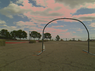
Original Image from Webcam
As with the cone detection system earlier, we use a standard USB webcam with a pipeline that consists of part OpenCV primitives and part custom detection routines. The output of the algorithm is an estimated range and bearing (and their estimated errors) to any hoops that might be present in the current frame.
In the example below, I’ll show how the process works on the sample image to the right, taken from Savage Solder during the AVC 2013.
Details
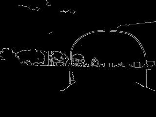
Edge Detection
Step A: First, we apply a Canny edge detection filter. We just use the default OpenCV “Canny” function. The thresholds are selected as part of our overall tuning process, although an initial guess was made based on what looked reasonable in some sample data sets.
Step B: As with the cone/barrel/ramp detection, we compute the distance transform. Here, since the objects of interest are thin lines, the distance transform lets us quickly compute how far away individual points are from that line. This is done using the OpenCV “distanceTransform” method.
Distance Transform
Step C: Using the original edge detected image, the OpenCV “findContours” method is used to identify all the contiguous lines. Contours which have fewer than a configurable number of points are dropped from the list of contours.
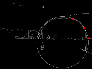
Step D: Now comes the first key part of the algorithm. At this point, we pick a random contour from our list of valid ones, then pick three random points on that contour. A circle is drawn circumscribing through those three points, to create a “proto-hoop”. A number of preliminary checks are run, if any of them fail, the proto-hoop is discarded and another sample is selected:
A Single Sampled Circle
Are all 3 points on the upper half of the circle?
Is the upper half of the circle entirely in the visual frame?
Is the center of the circle above a configurable minimum height?
Is the radius larger than a configurable minimum size?
If all the checks pass, then the circle is passed on to the next step.
Step E: At this point, we have a proto-hoop drawn in the image, but it might be three points that touched a square building, or a cloud, or a few people practicing their cheerleading. To distinguish these cases, we evaluate a support metric to determine how likely it is actually a hoop. To do so, we step through each pixel in the upper half of the circle in a clockwise manner. For each pixel, we compute two separate metrics which are later summed together. For clarity, the metric is defined such that smaller is better.
The square of the distance from that point on the circle to the nearest edge pixel. This prefers circles which are close to edges for most of their path.
The square root of the distance minus the square root of the previous point’s distance. This portion of the metric penalizes circles which are near very jagged edges. This is intended to penalize shapes like trees which are often circular-ish, but not very smooth.
If the support metric is too large for a given circle, then that circle is dropped and another sample is chosen.
Step F: Go back to step D and repeat a couple of hundred times.
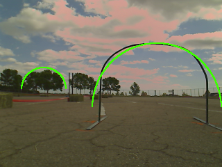
Step G: Finally, before reporting potential hoops, a last pass is taken. The proto-hoops are examined in order from best support to worst support. For each one, a local optimization function is run to find a nearby circle center and radius which improves the overall support. Then, for the first proto-hoop, it is just added to the output list. For subsequent hoops, they are compared against previously reported ones, and circles that substantially overlap are discarded as likely false positives.
Final Result: Two Detections
At this final stage, there are now a set of curated hoop detections for the given frame! The results are passed up to the tracker module, which correlates targets from frame to frame, discarding ones that don’t behave like a hoop should over time.
Results and Future Work
We only got the detector working with reasonable quality 2 or 3 weeks before the competition, so our corpus of images was not that large. However, in the dataset we do have, it is able to reliably detect the hoop out to about 6 meters of range with a manageable level of false positives. The table below shows the performance we had measured using data we took at our local testing sites.
Range (m)
Detections
False Detections
2-4
100% (18)
5.3% (1)
4-6
76% (16)
61% (25)
6-8
23% (16)
73% (14)
While the false positive level might seem high, the subsequent tracking is able to cope as the false positives tend to be randomly scattered about, and thus don’t form stable tracks from frame to frame. The detection rate within 6 meters is high enough that real hoops are detected 3 out of 4 times, which lets them be tracked just fine.
This approach seemed to work relatively well, although we had a relatively smaller corpus size compared to barrels and ramps. For future AVC competitions, we will likely use the same or similar technique, but trained on a larger dataset to avoid systematic failures like hoop shaped clouds, trees, or buildings.
We ran Savage Solder in two competitions this spring, Robomagellan in Robogames 2013, and the Sparkfun Autonomous Vehicle Competition 2013. In neither contest did we fare particularly well, especially given the level of preparation we put in. I’ll describe our results here, along with a little analysis from each event.
Robogames 2013 Robomagellan
Robogames 2013
In brief, the Robomagellan event requires that your robot touch a target orange traffic cone. It’s made harder because the cone can be in an arbitrary outdoor environment, with challenging terrain, changing features, people, GPS obstructions and the like. Your robot can achieve time deductions by touching other “bonus” cones. You get 3 runs, and your score is the best of the three.
Savage Solder only made two runs this year. A summary of the failure modes:
First Run: After touching the 25% bonus cone, our u-blox GPS decided to have a slew event, moving 20m away from where the car was. This resulted in the early termination of our run when the car hit a trash can. Our Robomagellan code has no obstacle avoidance, and it thought this was the final cone, so this ended our run.
Second Run: After the competition had started, the event center’s groundskeepers decided to start locating some picnic tables on the competition area. They placed one right in the middle of our surveyed path about 30s before we had to start. To change the plan, our robomagellan code at that time required surveying a series of waypoints, which we could not do in that short a time. The car got unlucky, clipped the side of the table enough to make it think it hit a cone, then reversed. When it reversed, it got hung up on the picnic table, burning out our ESC. We had no spare ESCs, so that ended our Robomagellan event.
Sparkfun AVC 2013
Sparkfun AVC 2013
The Sparkfun Autonomous Vehicle Competition, held for the last couple of years, requires the robot to drive around a loop course. Bonus points are awarded for passing through a medium sized metal hoop and jumping over a ramp. This year, the overall score was the sum total of three runs.
After our dissapointing Robomagellan performance, we doubled down for Sparkfun AVC. We replaced our ESC and got spares… of nearly everything. We built a ramp, hoop, and obtained barrels. The two weekends before the event the car was autonomously completing our practice course 100% of the time including hitting both the ramp and the jump about 90%-95% of the time over maybe a hundred runs.
How did this translate into our competition performance? We completed one run, failed after the second corner on the second run, and failed after the first corner on the third run. End result: not so hot.
First Run: This run was flawless. We set our speed at 11mph, on the theory that we completed most of our testing there, and we didn’t know how fast or successful at hitting the props the other teams would be.
Second Run: Here, after seeing Netburner’s fast run we increased our maximum speed to 15mph to shave some time off. This speed didn’t end up being a problem, aside from Netburner rear ending us going into the second turn harmlessly – but the clouds were a problem. When homing on the hoop, our hoop detector got a glimpse of some very hoop shaped clouds off in the distance and went for them. This ended badly after it closelined itself, ran into a couple of haybales and the curb. This was the first time we had a false positive on clouds in all our testing.
Third Run: I went back to the image data in our first and second run, and updated our hoop detection constants to have the same detection rate, but weed out all the clouds. We went with a speed of 15mph again. However, right before we started, I noticed on our display that it was complaining that the GPS was not reporting data regularly. In fact, it was barely reporting data at all. As with Robomagellan and the picnic tables, this problem appeared right before the starting gun, so there was nothing we could do but start it and watch. And watch we did, as it collided with the fence after the first turn. The root cause: the u-blox doesn’t seem to be able to emit NMEA messages longer than 364 characters when run at 115200, and the thus the u-blox’s PUBX,3 NMEA message gets truncated once the GPS has more than about 19 satellites in its tracking filter. Our GPS interface software requires all the messages it uses to be valid (with checksums) before emitting a fix upstream, so it wasn’t reporting anything most of the time. Looking back at the data from all our Boston testing, hundreds of hours worth, this only happened for a very brief time, maybe 10s total, as we don’t have the same clear view of the sky as in Boulder.
Fixes
u-blox GPS slew: We have seemingly resolved this by using the RMS of the reported range residuals as a floor on the measurement noise of position into our Kalman filter. Since that change, u-blox slews, while they still happen, don’t significantly impact the trajectory of the car.
Last minute picnic tables: For AVC 2013 and beyond, we’ve switched from surveying points with a handheld GPS to drawing interpolated curves on satellite maps which need maybe a one time registration. This allows us to change paths quickly as necessary.
Hoop shaped cloud: This one we fixed at the event by tuning constants. We didn’t get our hoop detector working until about 3 weeks before the event, so our corpus of hoop images was relatively small. If we run Sparkfun AVC again, I’ll also create a larger corpus of hoop images including some fluffy cloud days.
u-blox limited NMEA length: Here we are switching to use the u-blox binary protocol, which has both has shorter messages and is presumably better tested by u-blox.
Conclusions
Through both the spring competitions, we had 1 successful run out of 5. Of the 4 failed runs, 3 were from root causes we had never before seen, or had seen entirely too infrequently to diagnose. The 4th, (the u-blox slewing that caused our trash can hit), had been happening only every 4 or 5 robomagellan runs, so it was a known, but limited, risk.
Obviously, we are fixing all the individual failure modes that we observed. I am not sure what the larger lesson here is, other than that there are many many failure modes and the only way to find them all is through exhaustive testing. Maybe using more expensive components would have helped, as the cheap u-blox and our ESC with no overcurrent protection cost us 3 runs total (4 if you count our missed 3rd robomagellan run).
I suppose the ultimate conclusion is that building robots remains hard.
Savage Solder successfully participated in the superbly run Sparkfun AVC 2013 last weekend. The car ended up not running nearly as well as we had hoped, but we still had one flawless run which put us in third place in the doping class.
Sparkfun hasn’t posted a recap yet, but there are two videos online which mostly capture our one good run.
I will write up a post-mortem covering AVC 2013 and RoboGames Robomagellan 2013 in the coming weeks.
In part 1 and part 2, I covered the details of the localization solution we use on Savage Solder. To finish off, I’ll look at the areas we are exploring for future improvement.
u-blox 6 Position Errors
While in motion, our u-blox GPS can occasionally slew to an erroneous position that may be 20m away from ground truth, then slew back 20s later, even while reporting WAAS corrections, good HDOP and a large number of satellites. These slews of course confuse the localization algorithm, as they do not match the system dynamics at all. The estimation filter’s heading and position can diverge during these events.
One possible indication of these events can be found in the pseudo-range residuals the u-blox reports. The GPS receiver operates by measuring “pseudo-ranges” to each of the satellites it is tracking in the sky. In general, there are more ranges than necessary to determine both the receiver’s position and its clock bias at any point in time. Thus for any given position the receiver reports, there will be some error between what it thinks the range should be to each satellite, and what the actual measured pseudo-range was. This is reported as the “pseudo-range residual” via the NMEA GPGRS message.
During these error slew events, we have identified that the u-blox does generally report one or more of the residuals growing very large (sometimes more than 100m), then shrinking back down as the position corrects itself. This is even as it reports the same approximately constant horizontal position accuracy! For future competitions, such as Sparkfun AVC, we’re experimenting with using these residual measurements to de-weight GPS readings which are suspect. I’ve also put together the below video to describe the problem in more detail:
Error State Filter
The Kalman filter configuration we use now is a total state filter. In a total state localization filter, quantities such as the yaw rate are estimated as part of the filter, in addition to their error parameters. This makes the filter formulation straightforward, but results in an effective low pass filter applied on the yaw rate, as it is only updated through the Kalman filter measurement update step. Because of this filtering, in high dynamic maneuvers the heading can suffer from accuracy problems until the GPS is able to correct matters.
One alternate filter configuration, the “error-state filter”, estimates the error between a forward integrated solution and reality rather than estimating the solution directly. In this formulation, the error model parameters of the yaw rate gyro are included as states, but the yaw rate itself is not. This removes the low-pass filtering on the yaw rate, potentially improving filter response during fast maneuvering.
In part 1 I looked at the reasons why we use a state estimation filter for Savage Solder’s localization system and what the options were. This time, I’ll look at the specific measurements we take and the resulting states that we estimate along with some implementation details.
Measurements
Our localization system uses the following measurements:
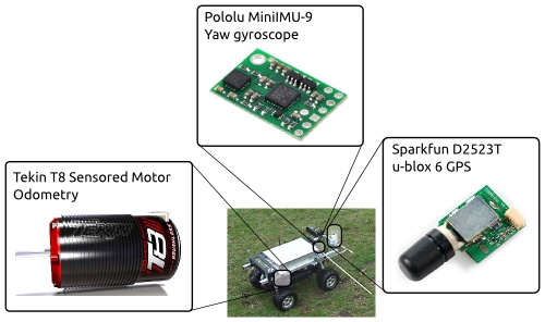
GPS: UTM (Universal Transverse Mercator) referenced position from a u-blox 6 GPS sampled at 4Hz
Odometer: We feed the sensors from our sensored brushless motor to an AVR microcontroller and count motor steps to measure odometry at 50Hz. This is not perfect, (for example, it suffers from backlash), but works reasonably well.
Each of these measurements is integrated into the state estimation filter at their natural rate. The filter only emits a solution on each IMU update, just to reduce the variability in the rest of the system.
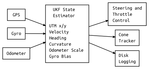
Savage Solder Localization Sensors
Estimated States
The Unscented Kalman Filter (UKF) estimates the following system states:
X/Y Position: The position is estimated in a UTM coordinate reference. We nominally estimate where a position under the center of the rear axle is, but the car is small enough that lever arms don’t really come into consideration.
Velocity Velocity is estimated assuming no lateral slip.
Heading: We assume that the car is always perfectly flat, and that the only orientation degree of freedom which matters is heading.
Curvature: We assume that the car moves in a car like way, and thus, given no change in steering input, it will drive in a circle.
Odometer Scale Factor: The only error term we estimate for the odometer is a scale factor. This is largely determined by errors in the diameter of the tires, but also is affected by the texture of the terrain that is being traversed.
Gyroscope Bias: Gyroscopes have many error factors which can be modeled. For our purposes, since we have accurate GPS most of the time, we get away with only estimating the bias of the gyroscope.
Constant Selection and Heuristics
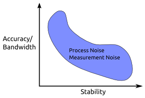
Kalman Filter Tuning Tradeoffs
When designing a state estimation filter, there are a lot of constants that need to be selected. For Kalman filters, you need an initial covariance and process noise for all estimated states, and measurement noise for all dimensions of the measured values. By choosing a specific selection of constants, you can trade off between the bandwidth (performance or accuracy) of the filter, and its stability. Generally, if you make the filter more accurate, you increase the risk that the filter will become unstable if the system model or measurement models do not accurately track the real world.
For Savage Solder, we used a largely ad-hoc approach, with no rigorous backing for our constant selection. We picked process noises that roughly corresponded to the amount of system error we expected to see, and did the same with measurement noises. One exception was GPS measurement error. Since we are using a naive total state filter, and GPS measurements from cheap receivers are highly time correlated (because of their own internal estimation filters), there are a number of other factors to consider. If the GPS measurement is set too high in this formulation, heading cannot be estimated accurately. If it is set too low, the global position will jump around a lot with every GPS update. In no case is the filter’s assumption, that of a measurement corrupted purely by white noise, satisfied, so measurements noises that are too low also run the risk of filter divergence. We just picked a happy medium that tends to work well in our simulations and practice.
There are also a fair number of heuristics included. For instance, if we know the car is stopped from the odometer, we artificially fix the heading and curvature estimates and covariances. At least when it is driving under its own power, Savage Solder rarely rotates in place. Without holding these fixed, noise in the GPS and gyroscope can cause the estimated heading to drift with no bounds and the heading uncertainty to grow arbitrarily large.
Global and Local Coordinate System
As I mentioned early in part 1, different subsystems in Savage Solder have differing requirements for the state estimates they consume. Some, like global driving, want the estimate to be close to the globally correct position so that the car can drive close to a pre-surveyed path. Others, like cone tracking, would much rather have a locally consistent frame of reference that is divorced from global coordinates entirely.
We solve this by deriving a separate local coordinate estimate from the global estimate emitted by the UKF. This local estimate always starts at position 0, 0 with a heading of 0. At each time step, the velocity, heading, and curvature of the global solution are integrated forward. This results in an estimate which is by definition smooth, yet still is relatively accurate over short distances, as the velocity and heading inputs have full access to the sensor suite of the car.
Coming Up…
In the next, and final installment, I’ll look at some techniques we are, or want to be exploring to improve the localization solution on Savage Solder.
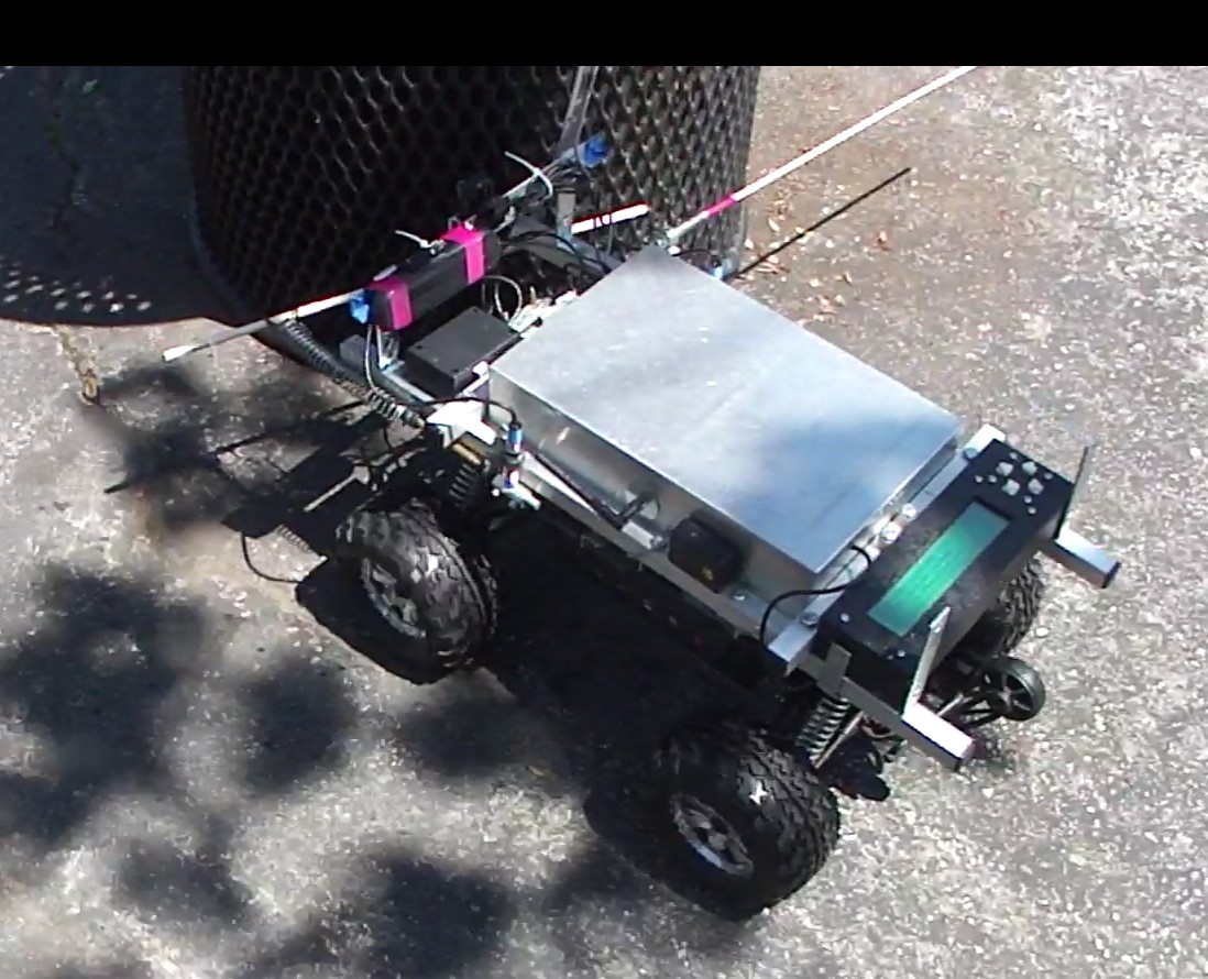
Today was the first day Savage Solder was firing on all cylinders in our Sparkfun AVC 2013 practice. We ran a pretty large number of circuits, and all systems seemed to be working pretty well, missing the hoop and ramp only a couple of times. Here is a video of a flawless run through the course at 11mph.
When it isn’t crashing into trash cans, Savage Solder uses a combination of several sensors to form accurate estimates about where it is in the world. This series describes the sensors and techniques that it uses to identify where it is in the world, providing data that is useful for the driving and cone tracking subsystems.
Inaccurate Localization
Principles
First, why does the car need to know where it is? Several other subsystems in Savage Solder rely on having accurate estimates of where the car is, measured in different ways. First, when driving to try and find a cone, it follows a path surveyed by GPS. In that case, the driving algorithm needs to know where the car is relative to the pre-surveyed path in order to select the appropriate steering and throttle commands. Here, absolute accuracy is most useful. We rely on surveyed paths to avoid obstacles, and the driving algorithm is relatively insensitive to position estimates that move around as GPS measurements change.
When moving in proximity to cones, the car needs a locally stable coordinate system in order to identify where the cone is relative to the car itself. For this, an estimate that is smooth is most important, as the car’s position relative to a cone can only change in a continuous manner.
For both of these cases, the localization subsystem on Savage Solder takes measurements from various sensors, and produces an estimate of the current position of the car. This estimate is updated on a regular basis, and fed to each other subsystem which needs to know where the car is.
Block diagram of Savage Solder’s localization system
Estimation
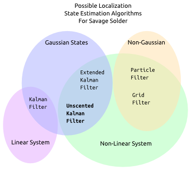
At the top level, Savage Solder uses a total-state unscented Kalman filter to incorporate measurements and produce localization estimates. Kalman filters are a class of algorithms which, given a series of noisy measurements of a system, estimate what the internal state variables the system are. In the localization problem, the noisy measurements are things like a GPS reading, a gyroscope measurement, or the value from an odometer, while the estimated state is perhaps the latitude and longitude of the vehicle along with its heading, heading rate and speed.
The Unscented Kalman filter is just one type of estimation algorithm. Traditionally, a designer would select it over other non-linear estimators when higher accuracy is required. As compared to estimators like the Extended Kalman Filter, it achieves this higher accuracy through an increase in computational cost.
For Savage Solder, our PC based computer platform has power to spare, so we chose the unscented Kalman filter (UKF) for a different reason. We used the UKF because it only requires numerical system models. Most non-linear Kalman filters, like the EKF, require analytical derivations of the partial derivatives of the system and measurement functions. These can be involved to create. When you want to change your design, and modify the estimated states or measurement variables, the process is slow and error prone. The UKF only requires a numerical definition of the system and measurement functions themselves. Because of this, we can experiment with different filter structures much more rapidly.
Options for Savage Solder’s localization estimation filter
Next Installment
In the next installment, I’ll look in more detail at the measurements we use, and the states that we estimate.
We got in our first day of autonomous practice this weekend for the Sparkfun AVC 2013. Some simple issues gave us some problems in the morning, but by the end of the day we had enough either resolved or worked around enough of them that we were achieving pretty good runs on a practice course. I’ve got video of our best run below, but first a couple of caveats:
We have a debugging creep at the start of the run to verify heading.
Our practice hoop wasn’t on the course. We don’t yet have a visual detector for the hoop, or our “hoop deflector” mounted on the car.
There is a debugging pause after it slaloms through the barrels, before it moves on to the ramp.
Today we took Savage Solder out to take some calibration image data of the various Sparkfun AVC obstacles and to experiment with manual navigation through an AVC style course. Unfortunately, we had some electronics failures with our replacement ESC that will take some repair. Before that though, we managed to collect a fair amount of useful data, and did a few jumps off the ramp. While not impossible, it looks to be pretty challenging. For small cars, the end of the ramp is actually pretty high. For large cars, the ramp is surprisingly narrow and was not trivial to hit when driving manually. This video is of the slowest run we dared do, higher speeds made better landings.