Sparkfun AVC: Visual Hoop Detection
While it caused us some grief during the actual competition, Savage Solder for the most part successfully used a vision based system to detect and track the bonus hoop necessary for extra points in this year’s Sparkfun AVC. The premise of our entry into the competition was a relatively cheap car, with nothing but cheap sensors. We compensated for our low accuracy GPS with a camera which allowed us to avoid barrels, and find the hoop and ramp at speed. Our barrel and hoop detection and tracking is basically unchanged from the cone detection we use in robomagellan style events. You can find a series describing it in part 1, part 2, and part 3. In this post, I’ll describe specifically our hoop detection algorithm, and give some results showing how well it performs on real world data.
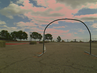
Original Image from Webcam
As with the cone detection system earlier, we use a standard USB webcam with a pipeline that consists of part OpenCV primitives and part custom detection routines. The output of the algorithm is an estimated range and bearing (and their estimated errors) to any hoops that might be present in the current frame.
In the example below, I’ll show how the process works on the sample image to the right, taken from Savage Solder during the AVC 2013.
Details
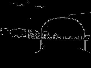
Edge Detection
Step A: First, we apply a Canny edge detection filter. We just use the default OpenCV “Canny” function. The thresholds are selected as part of our overall tuning process, although an initial guess was made based on what looked reasonable in some sample data sets.
Step B: As with the cone/barrel/ramp detection, we compute the distance transform. Here, since the objects of interest are thin lines, the distance transform lets us quickly compute how far away individual points are from that line. This is done using the OpenCV “distanceTransform” method.
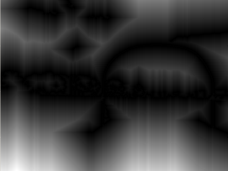
Distance Transform
Step C: Using the original edge detected image, the OpenCV “findContours” method is used to identify all the contiguous lines. Contours which have fewer than a configurable number of points are dropped from the list of contours.
Step D: Now comes the first key part of the algorithm. At this point, we pick a random contour from our list of valid ones, then pick three random points on that contour. A circle is drawn circumscribing through those three points, to create a “proto-hoop”. A number of preliminary checks are run, if any of them fail, the proto-hoop is discarded and another sample is selected:
A Single Sampled Circle
- Are all 3 points on the upper half of the circle?
- Is the upper half of the circle entirely in the visual frame?
- Is the center of the circle above a configurable minimum height?
- Is the radius larger than a configurable minimum size?
If all the checks pass, then the circle is passed on to the next step.
Step E: At this point, we have a proto-hoop drawn in the image, but it might be three points that touched a square building, or a cloud, or a few people practicing their cheerleading. To distinguish these cases, we evaluate a support metric to determine how likely it is actually a hoop. To do so, we step through each pixel in the upper half of the circle in a clockwise manner. For each pixel, we compute two separate metrics which are later summed together. For clarity, the metric is defined such that smaller is better.
- The square of the distance from that point on the circle to the nearest edge pixel. This prefers circles which are close to edges for most of their path.
- The square root of the distance minus the square root of the previous point’s distance. This portion of the metric penalizes circles which are near very jagged edges. This is intended to penalize shapes like trees which are often circular-ish, but not very smooth.
If the support metric is too large for a given circle, then that circle is dropped and another sample is chosen.
Step F: Go back to step D and repeat a couple of hundred times.
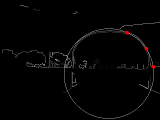
Step G: Finally, before reporting potential hoops, a last pass is taken. The proto-hoops are examined in order from best support to worst support. For each one, a local optimization function is run to find a nearby circle center and radius which improves the overall support. Then, for the first proto-hoop, it is just added to the output list. For subsequent hoops, they are compared against previously reported ones, and circles that substantially overlap are discarded as likely false positives.
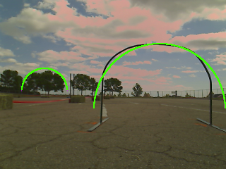
Final Result: Two Detections
At this final stage, there are now a set of curated hoop detections for the given frame! The results are passed up to the tracker module, which correlates targets from frame to frame, discarding ones that don’t behave like a hoop should over time.
Results and Future Work
We only got the detector working with reasonable quality 2 or 3 weeks before the competition, so our corpus of images was not that large. However, in the dataset we do have, it is able to reliably detect the hoop out to about 6 meters of range with a manageable level of false positives. The table below shows the performance we had measured using data we took at our local testing sites.
| Range (m) | Detections | False Detections |
|---|---|---|
| 2-4 | 100% (18) | 5.3% (1) |
| 4-6 | 76% (16) | 61% (25) |
| 6-8 | 23% (16) | 73% (14) |
While the false positive level might seem high, the subsequent tracking is able to cope as the false positives tend to be randomly scattered about, and thus don’t form stable tracks from frame to frame. The detection rate within 6 meters is high enough that real hoops are detected 3 out of 4 times, which lets them be tracked just fine.
This approach seemed to work relatively well, although we had a relatively smaller corpus size compared to barrels and ramps. For future AVC competitions, we will likely use the same or similar technique, but trained on a larger dataset to avoid systematic failures like hoop shaped clouds, trees, or buildings.