Savage Solder: Identifying Cones
Cone Tracking Block Diagram
One of the key aspects of our Savage Solder robomagellan solution is the ability to identify and track the orange traffic cones that serve as goal and bonus targets. Our approach to this is divided up into two parts, the first identification, the second tracking. They are roughly linked together with the block diagram to the right. Raw camera imagery is fed to the identification algorithm, which produces putative cones denoted by the bearing and range where they are estimated in the camera field of fiew. The tracking algorithm then takes those range and bearing estimates, along with the current navigation solution, and fuses them into a set of cartesian coordinate cones in the current neighborhood. Those local coordinates are then fed to the higher level race logic, which can decide to target or clip a cone if it is at the appropriate place in the script.
In this post, I’ll cover the Cone Identification Algorithm, listing out the individual steps within it.
Cone Detection Dataflow
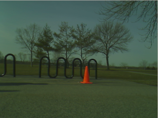
Original Image from Webcam
Our identification algorithm consists of a relatively simple image processing pipeline described below. We will work through a sample image starting from the source shown to the right:
Step A: First, we convert the image into the Hue Saturation Value color space, from the RGB values that our camera data source provides. In the HSV space, hue corresponds to color, and saturation and value determine how much color there is, and how white the color is. Since the traffic cones have a known color (orange), this helps us in later steps reject a lot of very unlikely regions of the visual field.
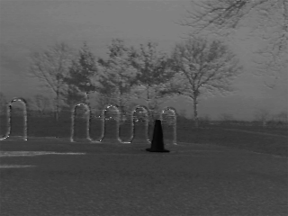
Hue Channel of HSV Transform
Step B: Second, we apply a limit filter to select only a subset of the hues and saturations, ignoring the value channel entirely. Both hue and saturation are parameterized by a center point and a range on either side of that center point which will be accepted. Since the hue values wrap around at 0, (red), we take care to select values on both sides of the center point. If the hue range does wrap around, we just do two limit operations, one for each side and merge the two together after the fact. The result of this process is a two color bitmap. It is black if there was no cone detected, white if there was a potential cone.
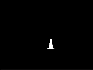
Bitmap with specific hue range selected
Step C: Next, we perform what OpenCV calls a “distance” transform on the resulting bitmap. This determines, for any given white pixel, how far it is to the nearest black pixel in any direction. Effectively, this will tell us how big any matched section is. It is not a terribly reliable indicator, as even a single black pixel in the middle of an otherwise large white area can result in halving the distance for all the pixels in that region. However, we use this to just discard regions that have a distance of 2 or less, which mostly throws away speckle noise. We also process each region in order of its distance score, so that we handle the biggest regions first.
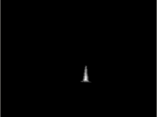
Distance metric
Step D: At this point, we iterate through the connected regions starting at those which contain the largest “distance” points. For each, we measure the bounding rectangle of the region, and from that caculate the aspect ratio and the fill percentage of the region. The aspect ratio is just the width divided by the height. The fill percentage is the percentage of pixels inside the bounding rectangle which were marked as being a cone. To be considered a valid cone, the aspect ratio and fill percentage must be within certain configured limits.
Step E: Finally, if the putative cone passed all the above checks, the bounding rectangle is used to estimate the bearing and distance. The bearing estimation is relatively straightforward. We assume our camera has no distortion and a field of view of 66 degrees. From there, the x coordinate of the bounding box center linearly relates to the bearing angle. Range is estimated using the total number of pixels detected in this region assuming the cone is a perfect sphere. We calibrated the size of the sphere to match the visible surface area of a cone. If the detected region abuts one of the edges of the camera image, then range is not emitted at all, as the range will be suspect due to some of the pixels being off screen. The very last step is to estimate the bearing and range uncertainty, which the detector generates for 1 standard deviation away from the mean. A guess for the bearing value is made assuming a fixed number of pixels of error in the x direction. For range, we assume that some percentage of the pixels will be missed, which would errnoneously make the cone seem farther away than it actually is.
Next Steps
One all the qualifying regions are processed, or the maximum number of visible cones are found (4 for our case), then we call this image done and record the outputs. Next, these values go on to the “cone tracker”, which generates Cartesian coordinate positions for each cone. I’ll discuss that module later.