Savage Solder: Selecting Constants for Image Processing
The final pieces of the cone detection and tracking system for Savage Solder are the tools we used to derive all the constants necessary for each of the algorithms. In part 1 (cone detector) and part 2 (cone tracker) I described how we first pick out possible range and bearings to cones in an image, and then take those range and bearings and turn them into a local Cartesian coordinate through the tracking process. As mentioned there, each of those stages has many tunable knobs.For the first stage, the following are the key parameters:
- Hue range - The window of hues to consider a pixel part of a valid cone.
- Saturation range - The range of saturation values to include.
- Minimum and maximum aspect ratio - Valid cone like objects are expected to be moderately narrow and tall.
- Minimum and maximum fill rate - If the image is crisp, most of the pixels in the bounding box, (but not all) should meet the filtering criteria.
Additionally, the cone tracker has its own set of parameters:
- Detection rate - given a real world cone at a certain distance, how likely are we to detect it?
- False positive rate - given a measurement at a specific range, how likely is it to be false?
- Range and bearing limits - At what range and bearing should we reject measurements.
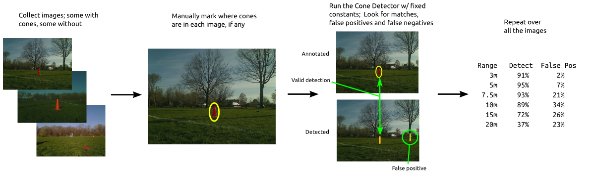
What we did in 2012, during the preparation for our first RoboMagellan, was take a lot of pictures of cones during our practice runs. Savage Solder normally is configured to save an image twice a second all the time it is running. These image datasets formed the basis of our ability to tune parameters and develop algorithms that would be robust in a wide range of conditions.
The basic idea we worked off was to create a metric for how good the system is, and then evaluate the metric over a set of data using our current algorithms and constants. You can then easily tweak the constants and algorithms as much as you want without running the car one bit and have good confidence that the results will be applicable to actual live runs.
Annotation Pipeline
Most of the metrics we wanted involved knowing where the cones actually were in the images. If we could just robustly identify cones in images programmatically, we wouldn’t really be worrying about this to begin with. So instead, we created a set of tools that let us rapidly mark, or annotate, images to indicate where the absolute ground truth of cones could be found. This is just a simple custom OpenCV program with some keyboard shortcuts that let us classify the cones in about 3000 images in a couple of hours. We selected images from varying times of day, angles, and lighting conditions, so that we would have a robust training set.
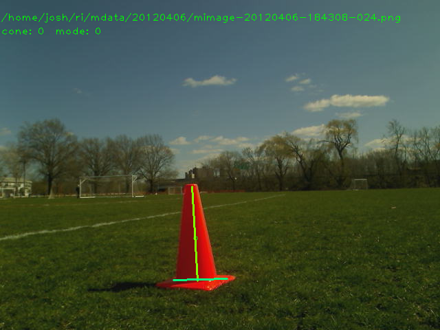
OpenCV Application for Annotation
Then, with a little wrapper script, we ran our cone detection algorithm over each of the frames. As mentioned in the on the cone detector, it outputs one or more range/bearing pairs to each of the prospective cones in the image. The quality metric then scores the cone detector based on accuracy of bearing and range to real cones, missed detections, and false detections. It also keeps histograms of each detection category by range. In the end, for a given set of cone detector parameters, we end up with a table that looks like the one below.
| Range | Detection Rate | False Positive Rate |
|---|---|---|
| 3m | 91% | 2% |
| 5m | 95% | 7% |
| 7.5m | 93% | 21% |
| 10m | 89% | 34% |
| 15m | 72% | 26% |
| 20m | 37% | 23% |
After each run over all the images, we would try changing the parameters to the cone detector, then seeing what the resultant table would like. Ideally, you have a much higher detection rate than false positive rate over the ranges you care about. The table above is actually the final one we were able to achieve for 2012, which allowed us to reliably sense cones at 15 meters of range using just our 640x480 stock webcam.