Mech Warfare Turret Design Preview
We’ve been hard at work on a Mech Warfare contender. Recently we got to a feature complete point on our turret design and build, and I put together a short video demonstrating its features. Enjoy!
We’ve been hard at work on a Mech Warfare contender. Recently we got to a feature complete point on our turret design and build, and I put together a short video demonstrating its features. Enjoy!
In Part 1 and Part 2, I described why we’re trying to measure localization accuracy, and the properties of a GPS receiver that allows us to do so. In this post, I’ll describe the technique we used to measure accuracy of our solution purely from recorded data, without needing to go back out to the field every time a change was made.
The technique we used to measure localization accuracy is somewhat similar to the Allan Variance plots used in part 2. Here, we take a large corpus of pre-recorded sensor data from the vehicle and re-run it through the localization solution. The trick is that for a given time window, the GPS updates are witheld from the filter, then at the end of the window, the difference between the estimated position and the measured GPS position is recorded. The cycle then starts anew at the current time, with the estimate being reset to the best possible one, and GPS denied until the next window end. Each sampled error is one data point showing how far off the localization solution can be after that much time with no GPS.
We expect this to be effective because, as the plots in part 2 showed, over short time windows, the average drift in the GPS is actually pretty small. For instance, the u-blox 6 on savage solder, within a 5s time window, will have drifted only about 0.6m with 95% confidence.
Once the results have been collated for a given time window, say 1s, we repeat the entire process for 2s, then 3s, etc. The curves this produces show how rapidly the position error in localization grows with time. The lower the value is at longer time intervals, that means the vehicle is more robust to GPS outages or drifts.
A plot of our 2013 AVC localization solution’s accuracy is shown below. It was measured over about 30 minutes of autonomous driving, mostly recorded in the weeks leading up to the 2013 AVC. I have superimposed on it the 68% and 95% confidence in the u-blox drift for reference. If the localization solution were perfect, we would expect the measured errors to approximately line up with the GPS drift over the same time interval.
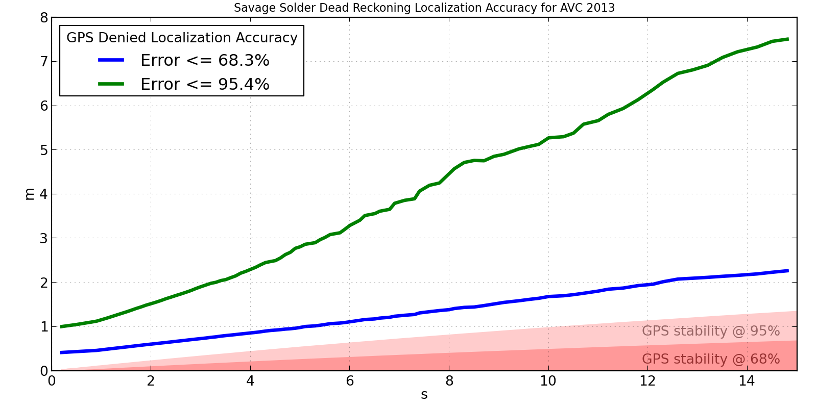
Savage Solder AVC 2013 Localization Accuracy
This shows that the accuracy isn’t terrible, but isn’t particularly great either. After 15 seconds, it is off by less than 2m two thirds of the time. However, in order to capture the best 95% of results, we have to look all the way out to 7.5m, which clearly isn’t too usable. For a course like the Sparkfun AVC one, you can roughly say that errors larger than 2 or 3 meters will result in a collision with something. This implies that Savage Solder can run for about 3 to 5 seconds with no GPS and be not terrible.
We have a couple of theories for where the largest sources of error are in the system as shown in the above plot:
Looking back at part 1, this technique measures up pretty well. It:
You can tweak the localization algorithms in software as many times as necessary, each time accurately assessing the results, and never once need to go out and actually drive the robot around.
I managed to clean up the python bindings to Gazebo I wrote when testing mech gaits in simulation, and have released them publicly as pygazebo.
All you have to do is:
pip install pygazebo
From the README, a simple example:
import eventlet
from pygazebo import Manager

manager = Manager()
publisher = manager.advertise('/gazebo/default/model/joint_cmd',
                              'gazebo.msgs.JointCmd')

message = pygazebo.msg.joint_cmd_pb2.JointCmd()
message.axis = 0
message.force = 1.0

while True:
    publisher.publish(message)
    eventlet.sleep(1.0)
and you’re off and ready to code!
In Part 1, I discussed how measuring the accuracy of a localization solution in a mobile robot is challenging, and some properties an ideal solution would have. This time, I’ll describe some of the properties of the GPS receiver Savage Solder uses, to motivate our mechanism for using it to measure localization accuracy.
The basic idea behind our approach is that the GPS mounted on Savage Solder, while relatively inaccurate in general, rarely has a very large error. And even when the error is large, it is usually only for a short window of time. Over time, these periods where the GPS has a lot of error come and go semi-randomly, which means that with enough data, they will tend to average out. To see how this works in a little more detail, let’s talk about the major sources of error that a GPS receiver can have.
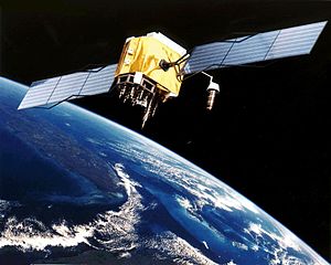
NASA rendering of GPS satellite
Geometry and clock error: At any given instant, only a subset of the GPS satellites are visible to a receiver, and those that are visible will have a configuration which introduces a source of error due to the process of triangulation. For instance, if all the visible satellites are in the same part of the sky, measuring ranges to the satellites will not tell you much about your absolute position. Secondly, each satellite may have differing errors in their onboard clocks, each of which translates directly in range measurement errors. Both of these error sources change relatively slowly with time.
Ephemeris and atmospheric effects: To estimate its location, a receiver must have precise knowledge of each satellite’s orbit, or ephemeris. While this orbit is known relatively precisely, every centimeter of error directly corresponds to positioning error on the ground. Ephemeris errors typically change slowly over time, as space weather isn’t as drastic as Boston weather. Atmospheric effects have similar properties when visible from the receiver, the ionosphere is the primary factor, as it causes delays in the signals propagating from the satellites to each receiver. Its effects also change relatively slowly with time.
Multipath and obstructions: When the line of sight to a receiver is blocked by a tree, building, person, vehicle, or the horizon, that can cause the signal to weaken enough to mis-register. The receiver can also pick up reflections of the actual satellite signal from any of the above. These reflected signals are called “multi-path”, and they cause the receiver to measure the additional length in the reflected path, instead of the true shortest path. As new satellites become available or are hidden, they can join or fall out of the solution. These errors can change rapidly for ground vehicles, where the line of sight to satellites can rapidly become clear or obstructed as it moves around.
Noise: Each measurement has some amount of random noise associated with it. Consumer receivers typically only measure the code phase, and not the carrier phase, so this measurement noise can be on the order of a meter or so for each satellite. It has mostly high frequency components.
Filtering: In order for the output to look more “reasonable”, most low-cost consumer receivers implement some sort of state estimation filtering before emitting any outputs. This smooths out noise components, and also smooths out rapid changes in multi-path or which satellites are used in the solution. As a result, the final position can often seem smooth, but as a result has more absolute error at any given instant.
To get an idea of the magnitude of each of these error types, we used a technique similar to Allan Variance to see the magnitude of error from the GPS solution in differing time domains. A long recording of reported GPS positions is made while the receiver is stationary. Then, it is divided up first into say consecutive 0.2s windows. Within each window the position is averaged, after which the change between consecutive windows is measured. These deltas represent how much the receiver’s absolute offset has drifted in that time period. For the 0.2s size, you can then see how much the offset changes on average, or how much it changes 95% of the time.
Once you’ve done that for the first window size, you increase the window size, say to 0.3s and repeat the whole process. You keep increasing the window size until you can only fit a few bins into the recorded trace.
What we expect to see is something like the following:
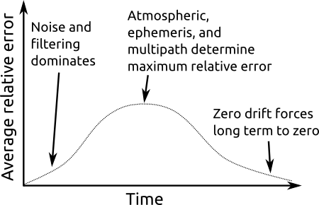
Typical GPS relative error plot
At very high frequencies (short time intervals), the filtering on the receiver renders the errors small. This means that on average, the position doesn’t change much over short intervals. Then, as the time interval gets up into the 5 to 60 minutes range, the error rapidly increases as we see the effects of atmospheric, ephemeris, and multipath errors become realized. Eventually, the error will peak, at a time interval which depends upon what the worst error contributor is. Finally, as the time grows to infinity, we would expect to see the error drop off, as averaging over such large time intervals tends to reveal the zero-drift property of GPS.
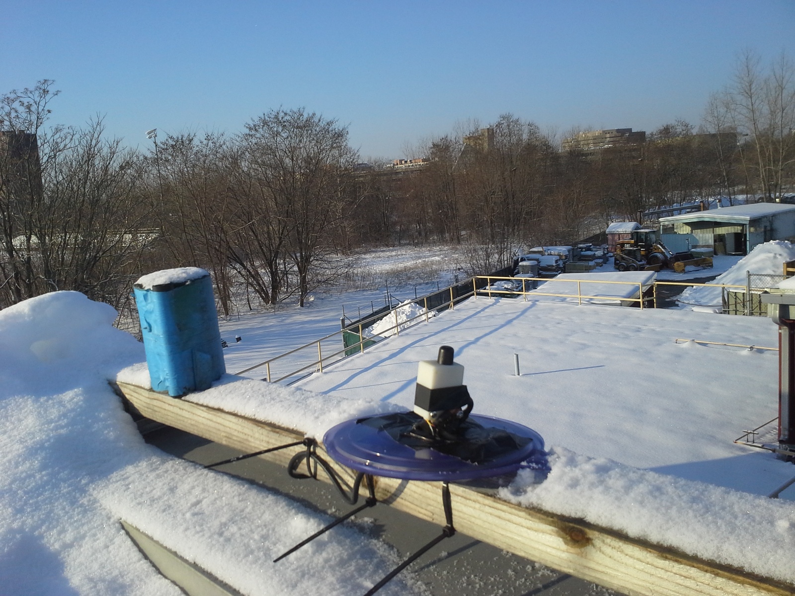
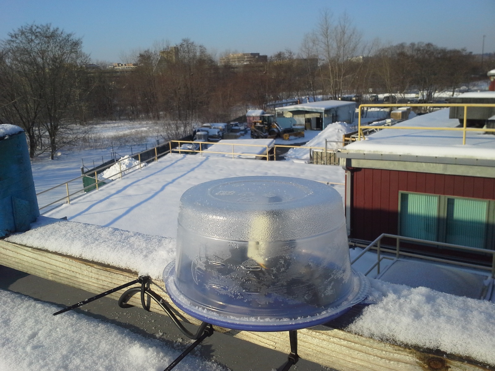
We ran this experiment on the u-blox 6 GPS used on Savage Solder and a high quality dual frequency receiver outfitted with Omnistar G2 as a reference. The u-blox was very crudely weatherized for long term outdoor recording with a disposable tupperware container. A recording at full data rate for each GPS was made over about 16 days of operation. Each GPS’s plot shows the median error and the maximum expected error for differing probabilities, which equate to about 1, 2, and 3 sigma on a normal distribution. (The non-weatherized u-blox was tested over a shorter duration and appeared to produce equivalent results.)
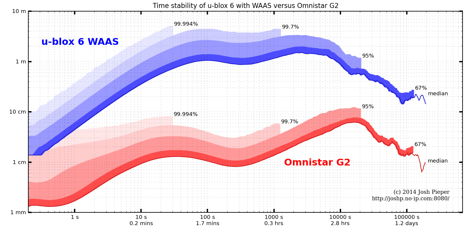
Time stability of u-blox 6 with WAAS versus Omnistar G2.
The data was taken while stationary on a rooftop with clear 360 degree view of the sky, and thus has best case visibility. Results on an AVC style course will be worse, since multi-path and obstructions will be constantly changing. Despite that, we can get some lower bounds on how good the system could possibly be from these results.
For instance, for a time commensurate with a Sparkfun AVC course run (about 45 seconds for a fast vehicle), the u-blox can be expected to drift around 2.2 meters with 95% confidence. The maximum drift over any interval with 95% confidence is around 3.3m, which implies that it is dicey to survey the course in ahead of time and expect the measurements to be useful. Also, the time required before averaging measurements actually starts to improve stability is pretty long. For the u-blox, it is around 1 hour, and even after looking at an entire day, the stability only gets down to around 24cm.
It is important to note that while the u-blox reports a GPS accuracy metric at any given time, it is usually extremely optimistic. For most of the above trace, the accuracy was reported as about 0.5m with a 1 sigma probability, when the measured absolute 1 sigma accuracy was clearly around 2m or more.
As a reference, the Omnistar G2 trace shows that yes, its performance is about 2 orders of magnitude better than the low-cost u-blox receiver. In these near-ideal conditions, it has a 95% confident maximum error of around 12cm, which means that it could be viable for hitting the hoop and ramp. However, as this is in ideal conditions, shading and multipath from the course, spectators, and other vehicles will certainly make actual results even worse.
In the next post, I’ll show how we used this knowledge of our GPS receiver’s error properties to measure the quality of our localization solution over short to medium time intervals.
Mikhail and I are considering fielding an entry into Mech Warfare this season. To evaluate different geometries and servo models, I tried setting up a simple simulation environment which would let us experiment without having to have a large variety of hardware on hand. While we’re not finished, I have a minimal first proof of concept working now, which I’ll describe briefly.
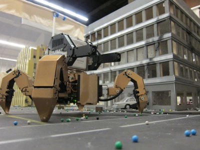
Immortal, competing in Mech Warfare at the KC Maker Faire
The simulator I’m using is Gazebo. It integrates several different rigid body physics engines, a 3D visualization environment, and a relatively simple file format for describing the configuration of robots. It uses a client server publish-subscribe model, where a central server maintains the physics simulation and any number of clients can connect to control or monitor individual models.
For gait generation, I’m starting with PyPose, which is a pose sequencer and inverse kinematics engine for the arbotiX controller, an open source Arduino compatible controller for Dynamixel servos. Specifically, the NUKE, or Nearly Universal Kinematics Engine, contains routines for generating a couple of different gait patterns for walking robots with lizard style legs.
The nominal workflow I wanted was to operate PyPose on a synthetic robot, simulated by Gazebo. I had to add a couple of pieces of software to make that happen.
To start, Gazebo doesn’t really have a documented protocol for interacting with its publish subscribe network. The primary way clients use it currently is through ROS. To make this work, I wrote up a simple python client library which implements the publish subscribe protocol using eventlet. This allows python applications to both subscribe to topics, as well as publish them.
Next, PyPose is very specialized to the Dynamixel servos and the arbotiX controller. Additionaly, from a gait generation perspective, it is effectively composed of effectively two independent parts. The first is an ahead of time pose sequencer and configuration tool written in python. The second, is a generated Arduino sketch which implements the actual gait when run on an AVR controller. The former, I hacked in a simple abstraction layer and connected it to the python Gazebo library. For the latter, I actually ported the generated C code back into python in order to test the generated gaits in simulation.
At the moment, I have only a rough proof of concept… the code is hacky, I haven’t yet simulated the physical characteristics of any particular servo, the physics model doesn’t seem quite right yet, and the Gazebo model consists of nothing but jointed rectangles with no textures. Despite that, in the video below, you can still see both PyPose manipulating the model, and the python gait generator operating it.
Next up, I’ll be trying to polish off the rough edges, and then try to evaluate the robot configuration variants I actually wanted to validate.
One of the challenges in developing a localization solution for a mobile robot is knowing when you are making things better versus making things worse. We felt this acutely when developing Savage Solder for the Sparkfun AVC event, especially as we were having intermittent GPS issues. Specifically, we are interested in knowing how well we can localize in the absence of GPS, or with poor GPS quality. In this series I’ll describe a new technique we’re using to make the process go a little faster as well as have a better understanding of just how accurate we are.
As a short refresher, the localization software in a mobile robot incorporates measurements from the robot’s sensors, and produces an estimate of where the robot is in one or more reference frames. Each of the sensors has errors that cause them to report non-ideal values. There can be many types of error, and the magnitudes of error can be relatively large. If a solution is good, it will report an accurate position even when the sensors aren’t so good.
A simple technique is make a change, let the car drive the course, and visually observe how close it was to the path that was planned. Lather, rinse, and repeat. Once you get into it, this technique breaks down rapidly:
It isn’t hard to see how the “simple” technique for improving a localization isn’t so simple after all.
Any solution you may want to use should have the following properties:
In the next post, I’ll begin developing the technique we’re using to measure localization accuracy and how it measures up to these properties.
Feedly just today came out with a Pro version with support for https support! Unfortunately, the one extension I rely on, FeedlyBackgroundTab hard-codes the URL to http://cloud.feedly.com. The required code change is trivial, just updating the list of allowed websites in the manifest file. To install it though, I wasn’t sure what to expect. First I tried just editing the file directly in my “~/.config/chromium” directory. That ended up not being successful. But then I noticed the little “Developer Mode” checkbox in the Chrome extensions page. Lo and behold, it can load unpacked extensions, or pack them for you!
Now if only the Omnibar would learn some awesomeness from the Awesome bar and I would all be set.
While it caused us some grief during the actual competition, Savage Solder for the most part successfully used a vision based system to detect and track the bonus hoop necessary for extra points in this year’s Sparkfun AVC. The premise of our entry into the competition was a relatively cheap car, with nothing but cheap sensors. We compensated for our low accuracy GPS with a camera which allowed us to avoid barrels, and find the hoop and ramp at speed. Our barrel and hoop detection and tracking is basically unchanged from the cone detection we use in robomagellan style events. You can find a series describing it in part 1, part 2, and part 3. In this post, I’ll describe specifically our hoop detection algorithm, and give some results showing how well it performs on real world data.
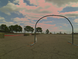
Original Image from Webcam
As with the cone detection system earlier, we use a standard USB webcam with a pipeline that consists of part OpenCV primitives and part custom detection routines. The output of the algorithm is an estimated range and bearing (and their estimated errors) to any hoops that might be present in the current frame.
In the example below, I’ll show how the process works on the sample image to the right, taken from Savage Solder during the AVC 2013.
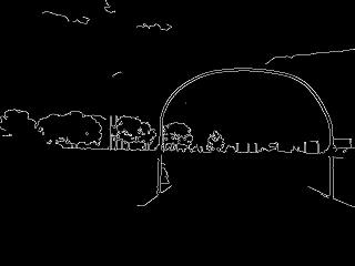
Edge Detection
Step A: First, we apply a Canny edge detection filter. We just use the default OpenCV “Canny” function. The thresholds are selected as part of our overall tuning process, although an initial guess was made based on what looked reasonable in some sample data sets.
Step B: As with the cone/barrel/ramp detection, we compute the distance transform. Here, since the objects of interest are thin lines, the distance transform lets us quickly compute how far away individual points are from that line. This is done using the OpenCV “distanceTransform” method.

Distance Transform
Step C: Using the original edge detected image, the OpenCV “findContours” method is used to identify all the contiguous lines. Contours which have fewer than a configurable number of points are dropped from the list of contours.
Step D: Now comes the first key part of the algorithm. At this point, we pick a random contour from our list of valid ones, then pick three random points on that contour. A circle is drawn circumscribing through those three points, to create a “proto-hoop”. A number of preliminary checks are run, if any of them fail, the proto-hoop is discarded and another sample is selected:
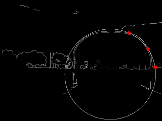
A Single Sampled Circle
If all the checks pass, then the circle is passed on to the next step.
Step E: At this point, we have a proto-hoop drawn in the image, but it might be three points that touched a square building, or a cloud, or a few people practicing their cheerleading. To distinguish these cases, we evaluate a support metric to determine how likely it is actually a hoop. To do so, we step through each pixel in the upper half of the circle in a clockwise manner. For each pixel, we compute two separate metrics which are later summed together. For clarity, the metric is defined such that smaller is better.
If the support metric is too large for a given circle, then that circle is dropped and another sample is chosen.
Step F: Go back to step D and repeat a couple of hundred times.
Step G: Finally, before reporting potential hoops, a last pass is taken. The proto-hoops are examined in order from best support to worst support. For each one, a local optimization function is run to find a nearby circle center and radius which improves the overall support. Then, for the first proto-hoop, it is just added to the output list. For subsequent hoops, they are compared against previously reported ones, and circles that substantially overlap are discarded as likely false positives.
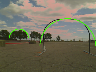
Final Result: Two Detections
At this final stage, there are now a set of curated hoop detections for the given frame! The results are passed up to the tracker module, which correlates targets from frame to frame, discarding ones that don’t behave like a hoop should over time.
We only got the detector working with reasonable quality 2 or 3 weeks before the competition, so our corpus of images was not that large. However, in the dataset we do have, it is able to reliably detect the hoop out to about 6 meters of range with a manageable level of false positives. The table below shows the performance we had measured using data we took at our local testing sites.
| Range (m) | Detections | False Detections |
|---|---|---|
| 2-4 | 100% (18) | 5.3% (1) |
| 4-6 | 76% (16) | 61% (25) |
| 6-8 | 23% (16) | 73% (14) |
While the false positive level might seem high, the subsequent tracking is able to cope as the false positives tend to be randomly scattered about, and thus don’t form stable tracks from frame to frame. The detection rate within 6 meters is high enough that real hoops are detected 3 out of 4 times, which lets them be tracked just fine.
This approach seemed to work relatively well, although we had a relatively smaller corpus size compared to barrels and ramps. For future AVC competitions, we will likely use the same or similar technique, but trained on a larger dataset to avoid systematic failures like hoop shaped clouds, trees, or buildings.
We ran Savage Solder in two competitions this spring, Robomagellan in Robogames 2013, and the Sparkfun Autonomous Vehicle Competition 2013. In neither contest did we fare particularly well, especially given the level of preparation we put in. I’ll describe our results here, along with a little analysis from each event.

Robogames 2013
In brief, the Robomagellan event requires that your robot touch a target orange traffic cone. It’s made harder because the cone can be in an arbitrary outdoor environment, with challenging terrain, changing features, people, GPS obstructions and the like. Your robot can achieve time deductions by touching other “bonus” cones. You get 3 runs, and your score is the best of the three.
Savage Solder only made two runs this year. A summary of the failure modes:
Sparkfun AVC 2013
The Sparkfun Autonomous Vehicle Competition, held for the last couple of years, requires the robot to drive around a loop course. Bonus points are awarded for passing through a medium sized metal hoop and jumping over a ramp. This year, the overall score was the sum total of three runs.
After our dissapointing Robomagellan performance, we doubled down for Sparkfun AVC. We replaced our ESC and got spares… of nearly everything. We built a ramp, hoop, and obtained barrels. The two weekends before the event the car was autonomously completing our practice course 100% of the time including hitting both the ramp and the jump about 90%-95% of the time over maybe a hundred runs.
How did this translate into our competition performance? We completed one run, failed after the second corner on the second run, and failed after the first corner on the third run. End result: not so hot.
Through both the spring competitions, we had 1 successful run out of 5. Of the 4 failed runs, 3 were from root causes we had never before seen, or had seen entirely too infrequently to diagnose. The 4th, (the u-blox slewing that caused our trash can hit), had been happening only every 4 or 5 robomagellan runs, so it was a known, but limited, risk.
Obviously, we are fixing all the individual failure modes that we observed. I am not sure what the larger lesson here is, other than that there are many many failure modes and the only way to find them all is through exhaustive testing. Maybe using more expensive components would have helped, as the cheap u-blox and our ESC with no overcurrent protection cost us 3 runs total (4 if you count our missed 3rd robomagellan run).
I suppose the ultimate conclusion is that building robots remains hard.
Savage Solder successfully participated in the superbly run Sparkfun AVC 2013 last weekend. The car ended up not running nearly as well as we had hoped, but we still had one flawless run which put us in third place in the doping class.
Sparkfun hasn’t posted a recap yet, but there are two videos online which mostly capture our one good run.
I will write up a post-mortem covering AVC 2013 and RoboGames Robomagellan 2013 in the coming weeks.