Savage Solder: Localization Part 3: Future Work
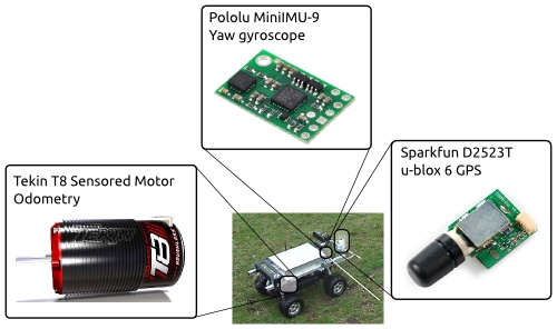
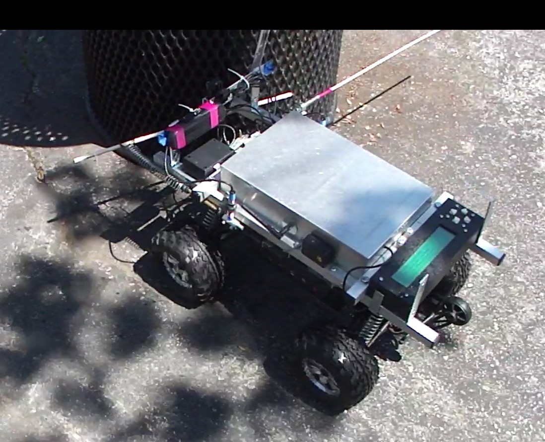
In part 1 and part 2, I covered the details of the localization solution we use on Savage Solder. To finish off, I’ll look at the areas we are exploring for future improvement.
u-blox 6 Position Errors
While in motion, our u-blox GPS can occasionally slew to an erroneous position that may be 20m away from ground truth, then slew back 20s later, even while reporting WAAS corrections, good HDOP and a large number of satellites. These slews of course confuse the localization algorithm, as they do not match the system dynamics at all. The estimation filter’s heading and position can diverge during these events.
One possible indication of these events can be found in the pseudo-range residuals the u-blox reports. The GPS receiver operates by measuring “pseudo-ranges” to each of the satellites it is tracking in the sky. In general, there are more ranges than necessary to determine both the receiver’s position and its clock bias at any point in time. Thus for any given position the receiver reports, there will be some error between what it thinks the range should be to each satellite, and what the actual measured pseudo-range was. This is reported as the “pseudo-range residual” via the NMEA GPGRS message.
During these error slew events, we have identified that the u-blox does generally report one or more of the residuals growing very large (sometimes more than 100m), then shrinking back down as the position corrects itself. This is even as it reports the same approximately constant horizontal position accuracy! For future competitions, such as Sparkfun AVC, we’re experimenting with using these residual measurements to de-weight GPS readings which are suspect. I’ve also put together the below video to describe the problem in more detail:
Error State Filter
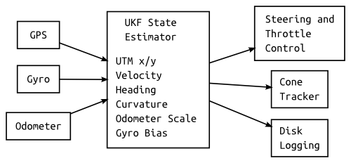
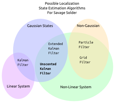
The Kalman filter configuration we use now is a total state filter. In a total state localization filter, quantities such as the yaw rate are estimated as part of the filter, in addition to their error parameters. This makes the filter formulation straightforward, but results in an effective low pass filter applied on the yaw rate, as it is only updated through the Kalman filter measurement update step. Because of this filtering, in high dynamic maneuvers the heading can suffer from accuracy problems until the GPS is able to correct matters.
One alternate filter configuration, the “error-state filter”, estimates the error between a forward integrated solution and reality rather than estimating the solution directly. In this formulation, the error model parameters of the yaw rate gyro are included as states, but the yaw rate itself is not. This removes the low-pass filtering on the yaw rate, potentially improving filter response during fast maneuvering.
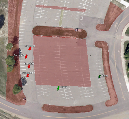
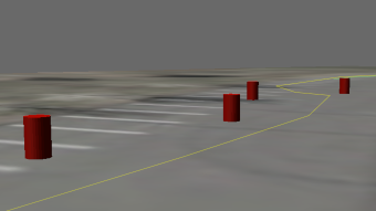 avc2013-barrel.blend
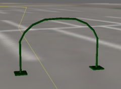 avc2013-hoop.blend
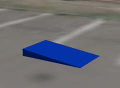 avc2013-ramp.blend