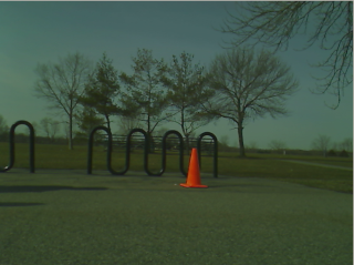
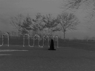
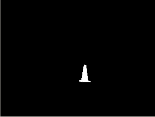
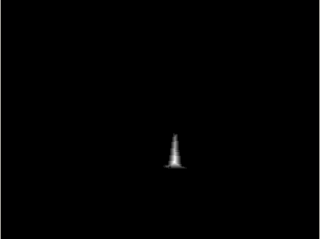
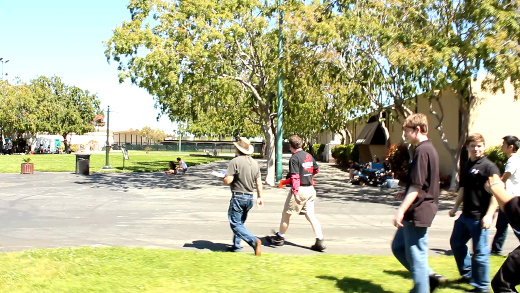
Last time I covered the techniques we use on Savage Solder to pick out orange traffic cones from webcam images in the “Cone Detector”. This time, I’ll look at the next stage in that pipeline, turning the range and bearing reported by the cone tracker into Cartesian coordinate estimates of where any given cone is.

Cone Tracker Overview

As mentioned last time, our “Cone Tracker” takes as input the range and bearing, (along with their uncertainties), from the cone detector. It also receives the current navigation state of the car. This includes things like the current estimate of geodetic position (latitude and longitude), current map position, (UTM easting and northing), and an unreferenced local coordinate system (x, y). For each of these, it reports the vehicle’s speed and heading.

I won’t go into the details of each of these coordinate systems here, but since the cone tracker actually only uses the local one, I can discuss it a bit. The local coordinate system on Savage Solder starts out at x,y=(0m,0m) with a heading of 0 degrees at the beginning of every run. As time progresses, the heading and position are updated primarily based on our onboard dead reckoning sensors. The local coordinate system is smooth, and never jumps for GPS updates. As a consequence, it isn’t really useful to compare positions in it from more than a minute or two apart, nor is it useful to do GPS based navigation. Fortunately, for cone tracking, from the time to when we see the cone to when we touch it is usually only a couple of seconds total over which time the local solution is very accurate.

Now, let’s cover some broad details of the implementation. The guts of our cone tracker consists of a bank of identical Kalman Filters. Each Kalman filter estimates the position of one particular cone and the error in that estimate. This lets the car keep around several possible cones that could be in sight at one time while still distinguishing them. By storing the cones in a local coordinate system, it allows for easy driving towards, or alongside, the cone and accurate speed control leading up to it. The position uncertainty could be used to control behavior, but we don’t bother in our current implementation.

New and Old Cones

Additionally, the tracker has to handle seeing new cones for the first time, and discarding cones that maybe were false detections in the cone detector. It does this by assigning each cone a “likelihood”, which is just a probability that the cone is a true detection. When data arrives that match the cone well, its likelihood is increased. When the available data doesn’t match the cone very well, or no cone is observed at all when one is expected, the likelihood is decreased.

If a range and bearing arrive which corresponds to no known cones, a new one is created with a relatively low likelihood. Then once it has reached a certain threshold, it is reported to the outside world as a valid target. Conversely, when an existing cone’s likelihood reaches a level which is too low, it is removed entirely on the thesis that it was actually a false detection to begin with.

More specifically, the likelihood update is handled using Bayes theorem. We have an empirically derived table showing, for our detector, the odds that a cone will be detected or a false one will be seen at various ranges. These are used to fill in the various probabilities in the equations.

Incorporating New Measurements

A “measurement” in this problem is simply the range and bearing that the cone detector reports. To incorporate a new measurement, the tracker looks through all the cones currently in its filter bank. For each, it computes a measure of the likelihood that the given cone could produce the current measurement. This is done using what’s called the Mahalanobis distance. The Mahalanobis distance is just a measure of how far away you are from an uncertain target in a multi-dimensional space.

If the best matching cone has a Mahalanobis distance small enough to count as valid, then the standard Kalman filter update equation is applied to that cone. If no cones match, then we create a new one as described above.

Scale Factor

One final detail, is that in addition to estimating the position of each cone, the tracker also estimates its “scale” as seen by the cone detector. The image based detector we use has the property that the range values are likely to have a fixed scale error for a number of reasons. One, the cones could actually be bigger or smaller than the regulation sized ones. Second, lighting conditions can sometimes cause a fraction of the cone to be not detected, which will result in the cone being seen as smaller than it actually is.

Since the range values are not correct, the position will be similarly off. This error isn’t as bad as it seems, since we (and most every RoboMagellan entrant), approach the cone in a straight line. Thus the position errors will always be directly towards or away from the robot, and as long as you keep moving, you’ll hit it eventually.

Savage Solder has two reasons to care. First, is that we decelerate from a high speed to an appropriate “bumping” speed with just a half meter to spare. Thus, if the cone is estimated as too close, we run the risk of colliding with it at an unsafe speed and damaging our front end. Secondly, we have a mode where the car can just “clip” the cone by driving alongside it and tapping it with a protruding stick. This allows us to avoid stopping entirely when the geometry allows it. However, if the position estimate is incorrect here, we might miss the cone entirely.

Final Process

To summarize, the cone tracker handles each new range and bearing with the following steps:

1. A cone detection results in a new range, bearing, and uncertainty measurement.
2. Existing cones in the Kalman filter bank are checked to see what the likelihood is each could have produced this measurement.
3. If one was likely enough, then:
   1. The position and scale factor are updated using the Kalman filter equations.
   2. The likelihood estimate is updated according to our current false positive and false negative estimates.
4. If none was likely enough, then a new cone is created with a position fixed at the exact position implied by the local navigation solution and the range and bearing.
5. Any cones which we had expected to see but didn’t have their likelihood decreased.
6. Any cones which have too low of a likelihood are removed.
7. Finally, all the cones which are close to the vehicle, and have a high enough likelihood are reported to the high level logic.

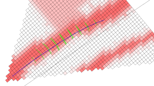
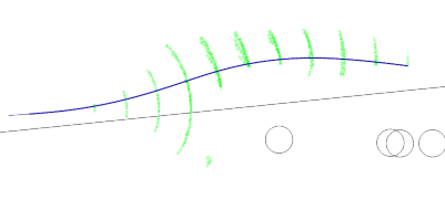
Caveats and Next Steps

One of the challenges with this approach is that there are a lot of constants to tune. I’ll cover the details in a later post, but for most of them we tried to find some way to empirically measure reasonable values for our application. Another problem was debugging. printf doesn’t cut it when you have this much geometry. For that, we created a number of custom debugging and visualization tools which help show what is going on in the system, some of which I’ll cover later too.

One of the key aspects of our Savage Solder robomagellan solution is the ability to identify and track the orange traffic cones that serve as goal and bonus targets. Our approach to this is divided up into two parts, the first identification, the second tracking. They are roughly linked together with the block diagram to the right. Raw camera imagery is fed to the identification algorithm, which produces putative cones denoted by the bearing and range where they are estimated in the camera field of fiew. The tracking algorithm then takes those range and bearing estimates, along with the current navigation solution, and fuses them into a set of cartesian coordinate cones in the current neighborhood. Those local coordinates are then fed to the higher level race logic, which can decide to target or clip a cone if it is at the appropriate place in the script.

In this post, I’ll cover the Cone Identification Algorithm, listing out the individual steps within it.

Cone Detection Dataflow

Our identification algorithm consists of a relatively simple image processing pipeline described below. We will work through a sample image starting from the source shown to the right:

Step A: First, we convert the image into the Hue Saturation Value color space, from the RGB values that our camera data source provides. In the HSV space, hue corresponds to color, and saturation and value determine how much color there is, and how white the color is. Since the traffic cones have a known color (orange), this helps us in later steps reject a lot of very unlikely regions of the visual field.

Step B: Second, we apply a limit filter to select only a subset of the hues and saturations, ignoring the value channel entirely. Both hue and saturation are parameterized by a center point and a range on either side of that center point which will be accepted. Since the hue values wrap around at 0, (red), we take care to select values on both sides of the center point. If the hue range does wrap around, we just do two limit operations, one for each side and merge the two together after the fact. The result of this process is a two color bitmap. It is black if there was no cone detected, white if there was a potential cone.

Step C: Next, we perform what OpenCV calls a “distance” transform on the resulting bitmap. This determines, for any given white pixel, how far it is to the nearest black pixel in any direction. Effectively, this will tell us how big any matched section is. It is not a terribly reliable indicator, as even a single black pixel in the middle of an otherwise large white area can result in halving the distance for all the pixels in that region. However, we use this to just discard regions that have a distance of 2 or less, which mostly throws away speckle noise. We also process each region in order of its distance score, so that we handle the biggest regions first.

Step D: At this point, we iterate through the connected regions starting at those which contain the largest “distance” points. For each, we measure the bounding rectangle of the region, and from that caculate the aspect ratio and the fill percentage of the region. The aspect ratio is just the width divided by the height. The fill percentage is the percentage of pixels inside the bounding rectangle which were marked as being a cone. To be considered a valid cone, the aspect ratio and fill percentage must be within certain configured limits.

Step E: Finally, if the putative cone passed all the above checks, the bounding rectangle is used to estimate the bearing and distance. The bearing estimation is relatively straightforward. We assume our camera has no distortion and a field of view of 66 degrees. From there, the x coordinate of the bounding box center linearly relates to the bearing angle. Range is estimated using the total number of pixels detected in this region assuming the cone is a perfect sphere. We calibrated the size of the sphere to match the visible surface area of a cone. If the detected region abuts one of the edges of the camera image, then range is not emitted at all, as the range will be suspect due to some of the pixels being off screen. The very last step is to estimate the bearing and range uncertainty, which the detector generates for 1 standard deviation away from the mean. A guess for the bearing value is made assuming a fixed number of pixels of error in the x direction. For range, we assume that some percentage of the pixels will be missed, which would errnoneously make the cone seem farther away than it actually is.

Next Steps

One all the qualifying regions are processed, or the maximum number of visible cones are found (4 for our case), then we call this image done and record the outputs. Next, these values go on to the “cone tracker”, which generates Cartesian coordinate positions for each cone. I’ll discuss that module later.

Earlier, we looked at how I used publicly available map data to create a simulation environment for Savage Solder, our robomagellan entry. Here, I’ll describe the process I used to source and manipulate the public GIS data into a form our simulation environment could use. There are two halves to this: the visible light imagery, and the elevation data used to build the 3D model.

Aerial Imagery

I started at the MASS GIS website located at: www.mass.gov. For Cambridge, that comes up with a tile map showing which tile corresponds to which area. From there, you can download MrSID data for the areas of interest.

The only free application I could find which adequately manipulated MrSID files was LizardTech’s GeoViewer, available for Windows only. I was able to use it to export a geotiff file containing the areas of interest.

Next, I used some tools from the GDAL open source software suite to manipulate the imagery (ubuntu package “gdal-bin”). The first was “gdalwarp”, which I used to do a preliminary projection into the Universal Transverse Mercator (UTM) projection. All of our vehicle and simulation software operates in this grid projection for simplicities sake.

gdalwarp -r cubic -t_srs '+proj=utm +zone=19 +datum=WGS84' \
  input.tif output_utm.tif

The next step was a little finicky. I used “listgeo” (from ubuntu “geotiff-bin”), to determine the UTM bounding coordinates of the image. Then I selected a new bounding area which, at the same pixel size, would result in an image with a power of two number of pixels in each direction. Then, I used “gdalwarp” to perform the final projection with those bounds.

listgeo output_utm.tif

gdalwarp -r cubic -t_srs '+proj=utm +zone=19 +datum=WGS84' \
  -te 323843.8 4694840.8 324458.2 4695455.2 \
  output_utm.tif final_image.tif

For the final step with the aerial imagery, I used “gdal_translate” to convert this .tif file into a .png.

gdal_translate -of png final_image.tif final_image.png

LIDAR Elevation

For the elevation side of things, I downloaded LIDAR data also from MASS GIS, on a site dedicated to a city of Boston high resolution LIDAR data drop. There you can use the index map to identify the appropriate tile(s) and download them individually.

For the LIDAR data, I used gdalwarp again for multiple purposes in one pass:

• To mosaic multiple LIDAR data files together.
• To project them into the UTM space.
• And finally, to crop and scale the final image to a known size and resolution.

The resulting gdalwarp command looks like:

gdalwarp -r cubic -t_srs '+proj=utm +zone=19 +datum=WGS84' \
  -te 323843.8 4694840.8 324458.2 4695455.2 -ts 1025 1025 \
  lidar_input_*.tif lidar_output.tif

Where the UTM bounds are the same ones used for reprojecting the aerial imagery. Our simulation environment requires a terrain map be sized to an even power of 2 plus 1, so here 1025 is chosen.

Finally, this tif file (which is still in floating point format), can be converted to a discrete .png using gdal_translate. I use “tifffile” from the ubuntu package “tifffile” to determine the minimum and maximum elevation to capture as much dynamic range as possible. In this case, the elevations run from about 0m above sea level to 50m.

gdal_translate -of png -scale 0 50 lidar_output.tif lidar_output.png

Last time working with the racing helicopter’s camera system, I managed to capture a poor quality image from the camera. My next step was attempting to diagnose the problems with the image quality. However, before I could do so, I ran into another problem with signal integrity in my breadboard setup.

The TI DM3730’s ISP with the 3.6 kernel is relatively sensitive to the quality of the pixel clock and vertical sync. If a single frame has the wrong number of pixels detected, the driver does not seem to be able to recover. This was a big problem for me, as the breadboard setup I have runs many of the 12MHz signal lines over 24 gauge wire springing around a breadboard. What I found was that I was only intermittently able to get the ISP to capture data, and eventually it got to a point where I could not get a single frame to capture despite all the wiggling I could attempt.

Rather than spending a large amount of time trying to tie up my breadboard wires just so, I instead just printed up a simple adapter board which contains all the level translation and keeps the signal paths short. This time, I tried printing it at oshpark.com, a competitor to batchpcb. The OV9650’s FFC connector has pads with a 7.8mil spacing, and batchpcb only supports 8.1mil, while oshpark has 6mil design rules. They also claim to ship faster, and are slightly cheaper.

The results were pretty good. From start to finish, it took 14 days to arrive, and the 3 boards appeared to have no major defects. My art had one minor error which required rework. The output enable pin on the level converters were tied to the wrong polarity, thus the lifted pins and blue wiring. Despite that, it appears to be working as intended.

Previously, I looked at how Savage Solder, our robomagellan entry, uses online replanning to avoid nearby cones. This time, I’ll cover the terrain oracle and how it integrates into the path planner.

For our simulation environment, we currently rely on digital elevation maps from the city of Cambridge along with aerial imagery of the environment. The simulator places the car in that fake world, and pretends to be each of the sensors that the car has. For Savage Solder, that is the IMU, the GPS, and the video camera.

In this first stage of staying on the pavement, we added an additional “oracle” sensor which has roughly the same field of view as the camera, but instead of reporting images, reports how fast the car can go at any point visible in the frame. The simulator gets this information from a hand-annotated map of the test area, where each pixel value corresponds to the maximum allowed speed. For example, below is downsampled aerial imagery of Danehy park in Cambridge, along with the hand annotated maximum speed map.

The locally referenced terrain data is fed into the online replanner. Currently, the maximum speed is just used as a penalty function, so that the car prefers to driver over terrain labeled with higher speeds. A sample online replanner output is shown below. Here, darker shades of red imply a higher maximum speed, and the black line is where the global GPS waypoints are in the current local reference frame. You can see the planned trajectory follow the red path despite it being offset some distance from the global trajectory. In practice, this will happen all the time, if nothing else because the GPS receiver on Savage Solder is comparatively low accuracy and often drifts by 3 or 4 meters in any direction.

As a caveat, the implementation now actually still drives at the speed programmed in by the global waypoints regardless of what the local maximum speeds are. The local sensor just modifies where it drives. Fixing that up is the immediate next step.

We hope this approach to also be useful for events like the Sparkfun AVC, where the traversable path is of the same size or narrower than the GPS accuracy.

As we gear towards higher speeds with our robomagellan entry, Savage Solder, one of the harder challenges is managing the terrain that the car drives on. In general, robomagellan competitions are held in campus or park like environments that consist of a mix of grass, pavement, wooded areas, and buildings. All of these terrain features affect how the car can navigate, and at what speeds. For instance, it shouldn’t drive into trees or buildings. In grass, the maximum speed should generally be lower than on pavement. Transition points may need an even lower speed as there could be a large bump where an area of grass ends, or where a manhole or other negative obstacle is present. Last year, we ran the car at about a maximum of 5mph, at which speed our platform can handle most all of the common event terrain features. However, as we go faster, we will want to make sure that if possible, the car stays on pavement, and avoids areas that could cause large problems.

We broke down our approach to tackle this problem into a number of discrete stages:

• **Online Replanning:**First, the car will run a local A* planner over short distances in the future. Initially, this will just avoid unexpected cones, since we are already tracking all cones in the vicinity of the car.
• Oracular Terrain:Next, we will hand annotate a map of one of our simulated environments, and create a synthetic “sensor” which reports the exact maximum speed in the robot’s local coordinate frame. This will feed into the local planner to keep the car on the path and at an appropriate speed.
• Derive Terrain from Camera:In the final stage, we will use our camera data to estimate what the maximum speed of visible terrain elements are, likely by using a simple color classifier.

We have implemented a rough prototype of the local replanner and have had success both in simulation and in the field with it. It operates as a hybrid A* planner with a primary state space consisting of x, y, heading, and velocity. The auxiliary, non-searched, states are just the previous steering command. At each time step, the planner searches a range of steering angle adjustments, as the steering servo on our platform requires about 1.5s to move from lock to lock. In a given plan time step only a small fraction of that motion is possible. The cost metric incorporates the rate at which the steering is changed, the distance away from the global waypoint path, and the proximity to any nearby cones.

In the picture above, the green vectors show the different possible vehicle positions and orientations that were considered, the black line shows the global waypoint path, and the blue line shows the best path explored so far. Each of the circles is an estimated cone (in this case there was actually only one cone, but the estimator hallucinated a few more in the vicinity).

Next, on this front, I’ll look into our efforts with an oracular terrain sensor.

Presume something is becoming more and more expensive, and in fact is approaching its record for being the most costly ever. Do you:

• a) Buy more
• b) Buy more
• c) Buy more
• d) Wait for it to become even more expensive, then buy more

One of the minor improvements we had planned for Savage Solder, our robomagellan entry, was to build a new enclosure for our LCD. I used this as an opportunity to experiment with some new manufacturing techniques in order to make something that was both more customized and still looked relatively professional.

In our previous incarnation of Savage Solder, our laptop was generally left closed while the car was in motion to save wear and tear on its hinges. During those periods, the LCD provided information on which stage of the plan the software was in, whether it was homing on a cone, and other auxiliary pieces of status. Watching the display as the car was moving added a lot of value over just looking at the results after the fact, as we had a lot more context.

My plan was to build an enclosure box using custom machined faces of ABS plastic, similar to Gary Chemelec’s approach documented at http://chemelec.com/Projects/Boxes/Boxes.htm. Basically, you cut sheets of ABS plastic into the correct dimensions for each edge, machine any holes for panel mounts, and then weld the result together with a plastic solvent.

Since I have been experimenting with some 3D printing, I drew up a 3D solid model of the display and an enclosure in FreeCAD. This gave me some confidence that I would be able to get the mounting hardware lined up properly with the display, and that the box dimensions would be big enough to encompass all the resulting hardware. In addition to the raw ABS box, a sheet of clear polycarbonate is inserted in between the LCD and the ABS cutout to better protect the LCD.

With that model, I ordered some ABS sheet from amazon, and went down to the Artisan’s Asylum to cut each side to the correct dimensions and machine the various holes. I used a jump shear to get each piece to roughly the correct dimension, then the Bridgeport mill with an Onsrud end mill bit to get each side square and to as close to the correct dimensions as I could. This portion of the process didn’t go as smoothly as I would have liked as I broke two mill bits making novice mistakes on the milling machine. I had planned on milling out the large LCD face using the mill as well, but instead of ordering a third mill bit, I just drilled a long series of holes using a standard ABS drill bit and completed the final cut and polish with a Dremel tool.

The welding process went relatively smoothly. I used an ABS glue compound that was a mixture of MEK (methyl ethyl ketone) and acetone and worked one edge at a time. The first edge was clamped to a square aluminum tube for alignment, the others self aligned against the already installed edges.

For the buttons on the right side of the display, I built a small backing board with a few momentary contact switches, then 3D printed a set of plastic buttons to fit into the front face holes that would be captured between the front face and the momentary contact switch. I used small bits of sandpaper to finish the face holes so that the buttons would have a snug, but freely moving fit.

The LCD itself was a 40x4 character version that Mikhail had previously developed an ATTiny hand built board to convert to RS232. The hand built board wouldn’t fit easily in the enclosure, so I drew up a PCB based on an ATMega32U4 which would go straight to USB, take up a bit less space, and use up some of the old parts I have lying around the lab. There were only two minor problems bringing up that board when it arrived. First, I did not realize that PORTF on the ATMega32U4 comes from the factory reserved for JTAG, where I was expecting it to be immediately available for GPIO. You can select the mode either with a boot fuse, or by configuring appropriate registers in software. Second, the LCD didn’t have any documentation, and at the time I didn’t have the source code to the original controller, so I mostly guessed at the HD44780 pinout, with the assumption that I could change things around in firmware later if things proved wrong. My guesses were actually mostly correct, but I got the ordering of the HD44780’s 4 data pins mixed up, so some bit re-arranging was required in the AVR that I hadn’t intended.

The final enclosure is pictured below, hopefully soon I will have pictures of it mounted on Savage Solder itself!

In the last post on my autonomous racing helicopter I managed to get the OV9650 camera communicating in a most basic way over the I2C bus. In order to actually capture images from it, the next step is to get a linux kernel driver going which can connect up the DM3730’s ISP (Image Signal Processor) hardware and route the resulting data into user space.

After some preliminary investigation, I found the first major problem. In the linux tree as of 3.6, there is a convenient abstraction in the video4linux2 (V4L2) universe for system on chips where the video device as a whole can represent the entire video capture chain, but each new “sensor” only needs a subdevice created for it. And there are in fact a lot of sensors already existing in the mainline kernel tree, including one for the very related OV9640 camera sensor. The downside however, is that there are two competing frameworks that sensor drivers can be written to, the “soc-camera” framework and the raw video4linux2 subdevice API. Sensors written for these two frameworks are incompatible, and from what I’ve seen, each platform supports only one of the frameworks. Of course, the omap3 platform which is used in the DM3730 only supports the video4linux2 API whereas all the similar sensors are written for the “soc-camera” framework!

Laurent Pinchart, a V4L2 developer has been working on this effort some, but I had a hard time locating a canonical description of the current state of affairs. Possibly the closest thing to a state of the soc-camera/v4l2 subdev universe can be found in this mailing list post:

Subject: Re: hacking MT9P031 for i.mx
From: Laurent Pinchart <laurent.pinchart@xxxxxxxxxxxxxxxx>
Date: Fri, 12 Oct 2012 15:11:09 +0200

...

soc-camera already uses v4l2_subdev, but requires soc-camera specific support
in the sensor drivers. I've started working on a fix for that some time ago,
some cleanup patches have reached mainline but I haven't been able to complete
the work yet due to lack of time.

--
Regards,

Laurent Pinchart

Since I don’t have a lot of need to upstream this work, I took the easy route and started with an existing v4l2 subdevice sensor, specifically the mt9v034 which is in the ISEE git repository. I copied it and replaced the guts with the ov9640 “soc-camera” driver from the mainline kernel. After a number of iterations I was able to get a driver that compiled, and appeared to operate the chip.

To test, I have been using Laurent Pinchart’s media-ctl and yavta tools. The media controller framework provides a general way to configure the image pipelines on system on chips. With it, you can configure whether the sensor output flows through the preview engine or the scaler and in what order if any. yavta is just a simple command line tool to set and query V4L2 controls and do simple frame capture.

One of the first images with correct coloring is below. Single frame capture out of the box was recognizable, but the quality was pretty poor. Also, as more frames were captured, the images became more and more washed out, with all the pixel values approaching the same bright gray color. That problem I will tackle in a later post.