LCD Enclosure for Savage Solder
One of the minor improvements we had planned for Savage Solder, our robomagellan entry, was to build a new enclosure for our LCD. I used this as an opportunity to experiment with some new manufacturing techniques in order to make something that was both more customized and still looked relatively professional.
In our previous incarnation of Savage Solder, our laptop was generally left closed while the car was in motion to save wear and tear on its hinges. During those periods, the LCD provided information on which stage of the plan the software was in, whether it was homing on a cone, and other auxiliary pieces of status. Watching the display as the car was moving added a lot of value over just looking at the results after the fact, as we had a lot more context.
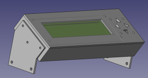
FeeCAD Model of Enclosure
My plan was to build an enclosure box using custom machined faces of ABS plastic, similar to Gary Chemelec’s approach documented at http://chemelec.com/Projects/Boxes/Boxes.htm. Basically, you cut sheets of ABS plastic into the correct dimensions for each edge, machine any holes for panel mounts, and then weld the result together with a plastic solvent.
Since I have been experimenting with some 3D printing, I drew up a 3D solid model of the display and an enclosure in FreeCAD. This gave me some confidence that I would be able to get the mounting hardware lined up properly with the display, and that the box dimensions would be big enough to encompass all the resulting hardware. In addition to the raw ABS box, a sheet of clear polycarbonate is inserted in between the LCD and the ABS cutout to better protect the LCD.
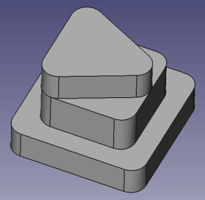
FreeCAD Model of Button
With that model, I ordered some ABS sheet from amazon, and went down to the Artisan’s Asylum to cut each side to the correct dimensions and machine the various holes. I used a jump shear to get each piece to roughly the correct dimension, then the Bridgeport mill with an Onsrud end mill bit to get each side square and to as close to the correct dimensions as I could. This portion of the process didn’t go as smoothly as I would have liked as I broke two mill bits making novice mistakes on the milling machine. I had planned on milling out the large LCD face using the mill as well, but instead of ordering a third mill bit, I just drilled a long series of holes using a standard ABS drill bit and completed the final cut and polish with a Dremel tool.
The welding process went relatively smoothly. I used an ABS glue compound that was a mixture of MEK (methyl ethyl ketone) and acetone and worked one edge at a time. The first edge was clamped to a square aluminum tube for alignment, the others self aligned against the already installed edges.
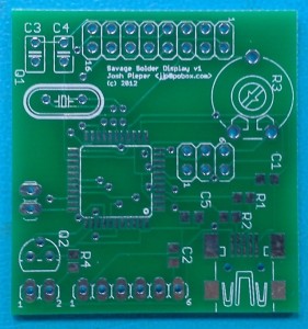
Unpopulated LCD Control Board
For the buttons on the right side of the display, I built a small backing board with a few momentary contact switches, then 3D printed a set of plastic buttons to fit into the front face holes that would be captured between the front face and the momentary contact switch. I used small bits of sandpaper to finish the face holes so that the buttons would have a snug, but freely moving fit.
The LCD itself was a 40x4 character version that Mikhail had previously developed an ATTiny hand built board to convert to RS232. The hand built board wouldn’t fit easily in the enclosure, so I drew up a PCB based on an ATMega32U4 which would go straight to USB, take up a bit less space, and use up some of the old parts I have lying around the lab. There were only two minor problems bringing up that board when it arrived. First, I did not realize that PORTF on the ATMega32U4 comes from the factory reserved for JTAG, where I was expecting it to be immediately available for GPIO. You can select the mode either with a boot fuse, or by configuring appropriate registers in software. Second, the LCD didn’t have any documentation, and at the time I didn’t have the source code to the original controller, so I mostly guessed at the HD44780 pinout, with the assumption that I could change things around in firmware later if things proved wrong. My guesses were actually mostly correct, but I got the ordering of the HD44780’s 4 data pins mixed up, so some bit re-arranging was required in the AVR that I hadn’t intended.
The final enclosure is pictured below, hopefully soon I will have pictures of it mounted on Savage Solder itself!
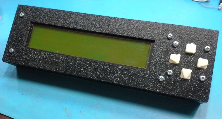
Final Savage Solder LCD Enclosure
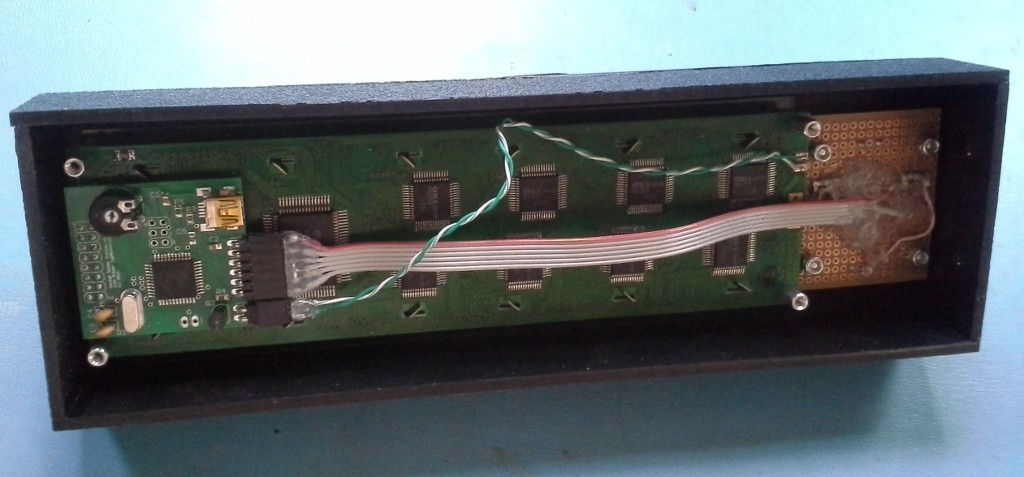
Enclosure Interior


 First, a little background. The motor controller on Savage Solder is the stock