Generating Usable Depth Maps from Aerial LIDAR Data
Earlier, we looked at how I used publicly available map data to create a simulation environment for Savage Solder, our robomagellan entry. Here, I’ll describe the process I used to source and manipulate the public GIS data into a form our simulation environment could use. There are two halves to this: the visible light imagery, and the elevation data used to build the 3D model.
Aerial Imagery
I started at the MASS GIS website located at: www.mass.gov. For Cambridge, that comes up with a tile map showing which tile corresponds to which area. From there, you can download MrSID data for the areas of interest.
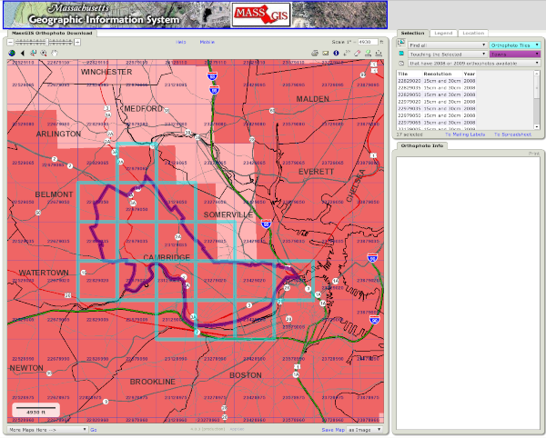
MASS GIS Aerial Tile Map
The only free application I could find which adequately manipulated MrSID files was LizardTech’s GeoViewer, available for Windows only. I was able to use it to export a geotiff file containing the areas of interest.
Next, I used some tools from the GDAL open source software suite to manipulate the imagery (ubuntu package “gdal-bin”). The first was “gdalwarp”, which I used to do a preliminary projection into the Universal Transverse Mercator (UTM) projection. All of our vehicle and simulation software operates in this grid projection for simplicities sake.
gdalwarp -r cubic -t_srs '+proj=utm +zone=19 +datum=WGS84' \
  input.tif output_utm.tif
The next step was a little finicky. I used “listgeo” (from ubuntu “geotiff-bin”), to determine the UTM bounding coordinates of the image. Then I selected a new bounding area which, at the same pixel size, would result in an image with a power of two number of pixels in each direction. Then, I used “gdalwarp” to perform the final projection with those bounds.
listgeo output_utm.tif

gdalwarp -r cubic -t_srs '+proj=utm +zone=19 +datum=WGS84' \
  -te 323843.8 4694840.8 324458.2 4695455.2 \
  output_utm.tif final_image.tif
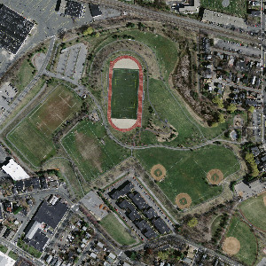
For the final step with the aerial imagery, I used “gdal_translate” to convert this .tif file into a .png.
gdal_translate -of png final_image.tif final_image.png

Final Downsampled Aerial Imagery
LIDAR Elevation
For the elevation side of things, I downloaded LIDAR data also from MASS GIS, on a site dedicated to a city of Boston high resolution LIDAR data drop. There you can use the index map to identify the appropriate tile(s) and download them individually.
For the LIDAR data, I used gdalwarp again for multiple purposes in one pass:
- To mosaic multiple LIDAR data files together.
- To project them into the UTM space.
- And finally, to crop and scale the final image to a known size and resolution.
The resulting gdalwarp command looks like:
gdalwarp -r cubic -t_srs '+proj=utm +zone=19 +datum=WGS84' \
  -te 323843.8 4694840.8 324458.2 4695455.2 -ts 1025 1025 \
  lidar_input_*.tif lidar_output.tif
Where the UTM bounds are the same ones used for reprojecting the aerial imagery. Our simulation environment requires a terrain map be sized to an even power of 2 plus 1, so here 1025 is chosen.
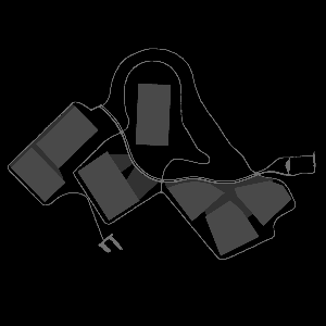
Finally, this tif file (which is still in floating point format), can be converted to a discrete .png using gdal_translate. I use “tifffile” from the ubuntu package “tifffile” to determine the minimum and maximum elevation to capture as much dynamic range as possible. In this case, the elevations run from about 0m above sea level to 50m.
gdal_translate -of png -scale 0 50 lidar_output.tif lidar_output.png
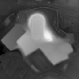
Final Downsampled LIDAR Elevation