In Part 1 and Part 2, I described why we’re trying to measure localization accuracy, and the properties of a GPS receiver that allows us to do so. In this post, I’ll describe the technique we used to measure accuracy of our solution purely from recorded data, without needing to go back out to the field every time a change was made.

Our solution

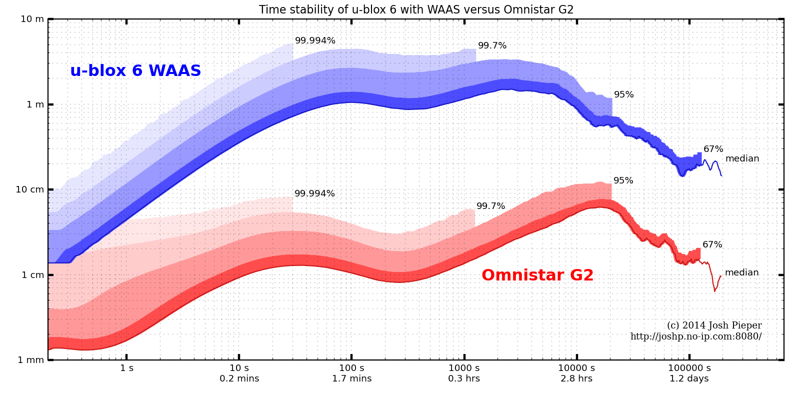
The technique we used to measure localization accuracy is somewhat similar to the Allan Variance plots used in part 2. Here, we take a large corpus of pre-recorded sensor data from the vehicle and re-run it through the localization solution. The trick is that for a given time window, the GPS updates are witheld from the filter, then at the end of the window, the difference between the estimated position and the measured GPS position is recorded. The cycle then starts anew at the current time, with the estimate being reset to the best possible one, and GPS denied until the next window end. Each sampled error is one data point showing how far off the localization solution can be after that much time with no GPS.

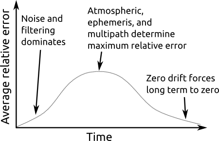
We expect this to be effective because, as the plots in part 2 showed, over short time windows, the average drift in the GPS is actually pretty small. For instance, the u-blox 6 on savage solder, within a 5s time window, will have drifted only about 0.6m with 95% confidence.

Once the results have been collated for a given time window, say 1s, we repeat the entire process for 2s, then 3s, etc. The curves this produces show how rapidly the position error in localization grows with time. The lower the value is at longer time intervals, that means the vehicle is more robust to GPS outages or drifts.

Results on Savage Solder’s 2013 AVC software

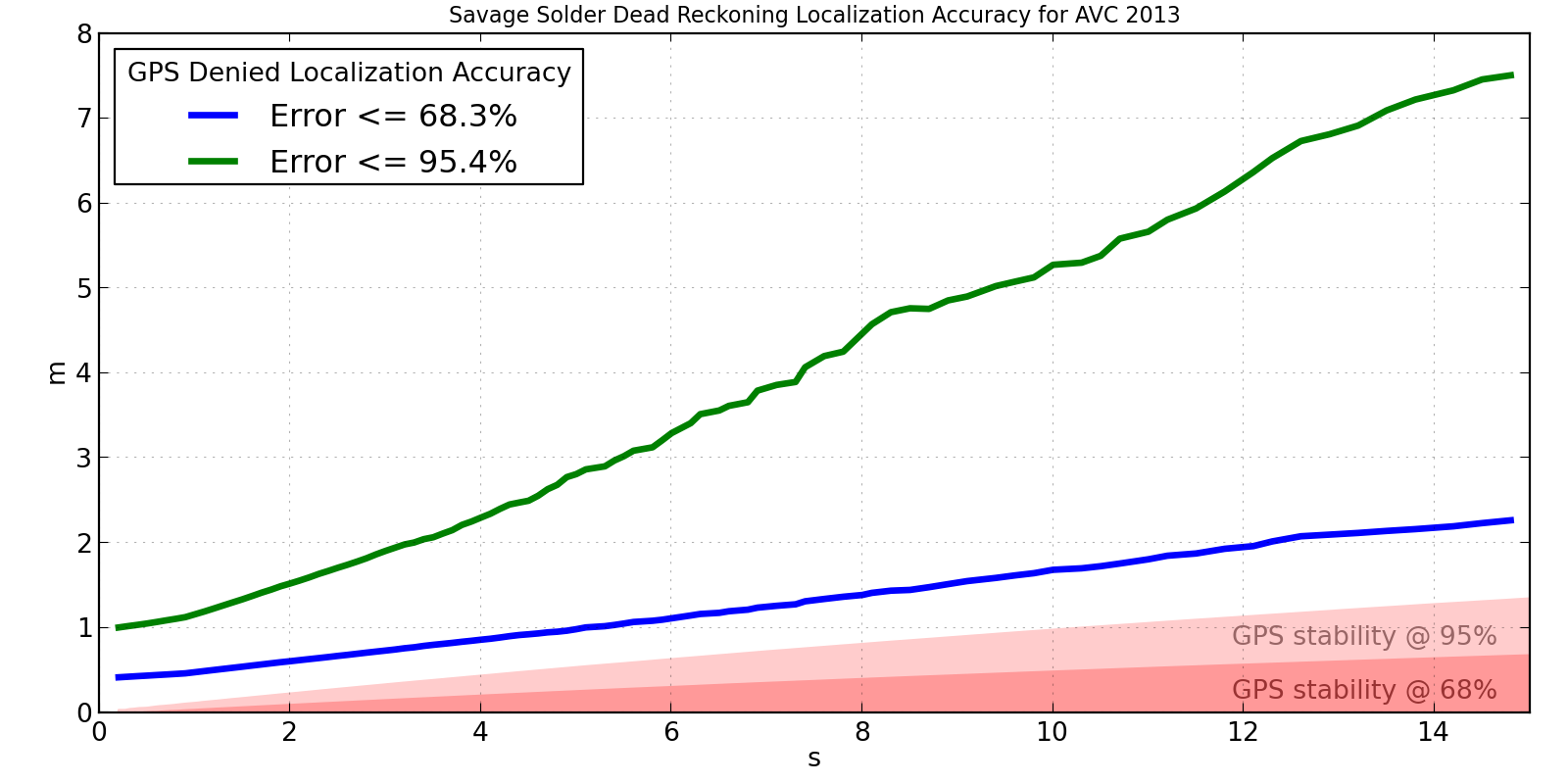
A plot of our 2013 AVC localization solution’s accuracy is shown below. It was measured over about 30 minutes of autonomous driving, mostly recorded in the weeks leading up to the 2013 AVC. I have superimposed on it the 68% and 95% confidence in the u-blox drift for reference. If the localization solution were perfect, we would expect the measured errors to approximately line up with the GPS drift over the same time interval.

This shows that the accuracy isn’t terrible, but isn’t particularly great either. After 15 seconds, it is off by less than 2m two thirds of the time. However, in order to capture the best 95% of results, we have to look all the way out to 7.5m, which clearly isn’t too usable. For a course like the Sparkfun AVC one, you can roughly say that errors larger than 2 or 3 meters will result in a collision with something. This implies that Savage Solder can run for about 3 to 5 seconds with no GPS and be not terrible.

We have a couple of theories for where the largest sources of error are in the system as shown in the above plot:

• Initial heading error: For all of these data sets, the car has only a very rough knowledge of its heading when starting out and all information about the heading comes from GPS. Even a small initial heading error will result in large position errors early in each run.
• Total state filter: As described before the localization solution used during 2013 was a total state Kalman filter. I expect that switching to an error state can improve the performance.
• Improved inertial sensors: This can’t strictly be tested after the fact, but there now exist easily obtainable higher quality gyroscopes and accelerometers than the Pololu MiniIMU v2 we used in 2013.

Recap of measuring localization accuracy

Looking back at part 1, this technique measures up pretty well. It:

1. requires only data recorded on the robot, it
2. provides hard numeric results (within the limits of the GPS’s short term drift), and it
3. requires no additional sensors

You can tweak the localization algorithms in software as many times as necessary, each time accurately assessing the results, and never once need to go out and actually drive the robot around.

In Part 1, I discussed how measuring the accuracy of a localization solution in a mobile robot is challenging, and some properties an ideal solution would have. This time, I’ll describe some of the properties of the GPS receiver Savage Solder uses, to motivate our mechanism for using it to measure localization accuracy.

Principles

The basic idea behind our approach is that the GPS mounted on Savage Solder, while relatively inaccurate in general, rarely has a very large error. And even when the error is large, it is usually only for a short window of time. Over time, these periods where the GPS has a lot of error come and go semi-randomly, which means that with enough data, they will tend to average out. To see how this works in a little more detail, let’s talk about the major sources of error that a GPS receiver can have.

Geometry and clock error: At any given instant, only a subset of the GPS satellites are visible to a receiver, and those that are visible will have a configuration which introduces a source of error due to the process of triangulation. For instance, if all the visible satellites are in the same part of the sky, measuring ranges to the satellites will not tell you much about your absolute position. Secondly, each satellite may have differing errors in their onboard clocks, each of which translates directly in range measurement errors. Both of these error sources change relatively slowly with time.

Ephemeris and atmospheric effects: To estimate its location, a receiver must have precise knowledge of each satellite’s orbit, or ephemeris. While this orbit is known relatively precisely, every centimeter of error directly corresponds to positioning error on the ground. Ephemeris errors typically change slowly over time, as space weather isn’t as drastic as Boston weather. Atmospheric effects have similar properties when visible from the receiver, the ionosphere is the primary factor, as it causes delays in the signals propagating from the satellites to each receiver. Its effects also change relatively slowly with time.

Multipath and obstructions: When the line of sight to a receiver is blocked by a tree, building, person, vehicle, or the horizon, that can cause the signal to weaken enough to mis-register. The receiver can also pick up reflections of the actual satellite signal from any of the above. These reflected signals are called “multi-path”, and they cause the receiver to measure the additional length in the reflected path, instead of the true shortest path. As new satellites become available or are hidden, they can join or fall out of the solution. These errors can change rapidly for ground vehicles, where the line of sight to satellites can rapidly become clear or obstructed as it moves around.

Noise: Each measurement has some amount of random noise associated with it. Consumer receivers typically only measure the code phase, and not the carrier phase, so this measurement noise can be on the order of a meter or so for each satellite. It has mostly high frequency components.

Filtering: In order for the output to look more “reasonable”, most low-cost consumer receivers implement some sort of state estimation filtering before emitting any outputs. This smooths out noise components, and also smooths out rapid changes in multi-path or which satellites are used in the solution. As a result, the final position can often seem smooth, but as a result has more absolute error at any given instant.

Windowed error measurement

To get an idea of the magnitude of each of these error types, we used a technique similar to Allan Variance to see the magnitude of error from the GPS solution in differing time domains. A long recording of reported GPS positions is made while the receiver is stationary. Then, it is divided up first into say consecutive 0.2s windows. Within each window the position is averaged, after which the change between consecutive windows is measured. These deltas represent how much the receiver’s absolute offset has drifted in that time period. For the 0.2s size, you can then see how much the offset changes on average, or how much it changes 95% of the time.

Once you’ve done that for the first window size, you increase the window size, say to 0.3s and repeat the whole process. You keep increasing the window size until you can only fit a few bins into the recorded trace.

What we expect to see is something like the following:

At very high frequencies (short time intervals), the filtering on the receiver renders the errors small. This means that on average, the position doesn’t change much over short intervals. Then, as the time interval gets up into the 5 to 60 minutes range, the error rapidly increases as we see the effects of atmospheric, ephemeris, and multipath errors become realized. Eventually, the error will peak, at a time interval which depends upon what the worst error contributor is. Finally, as the time grows to infinity, we would expect to see the error drop off, as averaging over such large time intervals tends to reveal the zero-drift property of GPS.

We ran this experiment on the u-blox 6 GPS used on Savage Solder and a high quality dual frequency receiver outfitted with Omnistar G2 as a reference. The u-blox was very crudely weatherized for long term outdoor recording with a disposable tupperware container. A recording at full data rate for each GPS was made over about 16 days of operation. Each GPS’s plot shows the median error and the maximum expected error for differing probabilities, which equate to about 1, 2, and 3 sigma on a normal distribution. (The non-weatherized u-blox was tested over a shorter duration and appeared to produce equivalent results.)

Analysis

The data was taken while stationary on a rooftop with clear 360 degree view of the sky, and thus has best case visibility. Results on an AVC style course will be worse, since multi-path and obstructions will be constantly changing. Despite that, we can get some lower bounds on how good the system could possibly be from these results.

For instance, for a time commensurate with a Sparkfun AVC course run (about 45 seconds for a fast vehicle), the u-blox can be expected to drift around 2.2 meters with 95% confidence. The maximum drift over any interval with 95% confidence is around 3.3m, which implies that it is dicey to survey the course in ahead of time and expect the measurements to be useful. Also, the time required before averaging measurements actually starts to improve stability is pretty long. For the u-blox, it is around 1 hour, and even after looking at an entire day, the stability only gets down to around 24cm.

It is important to note that while the u-blox reports a GPS accuracy metric at any given time, it is usually extremely optimistic. For most of the above trace, the accuracy was reported as about 0.5m with a 1 sigma probability, when the measured absolute 1 sigma accuracy was clearly around 2m or more.

As a reference, the Omnistar G2 trace shows that yes, its performance is about 2 orders of magnitude better than the low-cost u-blox receiver. In these near-ideal conditions, it has a 95% confident maximum error of around 12cm, which means that it could be viable for hitting the hoop and ramp. However, as this is in ideal conditions, shading and multipath from the course, spectators, and other vehicles will certainly make actual results even worse.

Using this

In the next post, I’ll show how we used this knowledge of our GPS receiver’s error properties to measure the quality of our localization solution over short to medium time intervals.